healthyverse_tsa
Time Series Analysis, Modeling and Forecasting of the Healthyverse Packages
Steven P. Sanderson II, MPH - Date: 2026-07-03
Introduction
This analysis follows a Nested Modeltime Workflow from modeltime
along with using the NNS package. I use this to monitor the
downloads of all of my packages:
Get Data
glimpse(downloads_tbl)
Rows: 183,083
Columns: 11
$ date      <date> 2020-11-23, 2020-11-23, 2020-11-23, 2020-11-23, 2020-11-23,…
$ time      <Period> 15H 36M 55S, 11H 26M 39S, 23H 34M 44S, 18H 39M 32S, 9H 0M…
$ date_time <dttm> 2020-11-23 15:36:55, 2020-11-23 11:26:39, 2020-11-23 23:34:…
$ size      <int> 4858294, 4858294, 4858301, 4858295, 361, 4863722, 4864794, 4…
$ r_version <chr> NA, "4.0.3", "3.5.3", "3.5.2", NA, NA, NA, NA, NA, NA, NA, N…
$ r_arch    <chr> NA, "x86_64", "x86_64", "x86_64", NA, NA, NA, NA, NA, NA, NA…
$ r_os      <chr> NA, "mingw32", "mingw32", "linux-gnu", NA, NA, NA, NA, NA, N…
$ package   <chr> "healthyR.data", "healthyR.data", "healthyR.data", "healthyR…
$ version   <chr> "1.0.0", "1.0.0", "1.0.0", "1.0.0", "1.0.0", "1.0.0", "1.0.0…
$ country   <chr> "US", "US", "US", "GB", "US", "US", "DE", "HK", "JP", "US", …
$ ip_id     <int> 2069, 2804, 78827, 27595, 90474, 90474, 42435, 74, 7655, 638…
The last day in the data set is 2026-07-01 23:53:43, the file was birthed on: 2025-10-31 10:47:59.603742, and at report knit time is 5841.1 hours old. Happy analyzing!
Now that we have our data lets take a look at it using the skimr
package.
skim(downloads_tbl)
| Name | downloads_tbl |
| Number of rows | 183083 |
| Number of columns | 11 |
| _______________________ | |
| Column type frequency: | |
| character | 6 |
| Date | 1 |
| numeric | 2 |
| POSIXct | 1 |
| Timespan | 1 |
| ________________________ | |
| Group variables | None |
Data summary
Variable type: character
| skim_variable | n_missing | complete_rate | min | max | empty | n_unique | whitespace |
|---|---|---|---|---|---|---|---|
| r_version | 137118 | 0.25 | 5 | 7 | 0 | 52 | 0 |
| r_arch | 137118 | 0.25 | 1 | 7 | 0 | 6 | 0 |
| r_os | 137118 | 0.25 | 7 | 19 | 0 | 30 | 0 |
| package | 0 | 1.00 | 7 | 13 | 0 | 8 | 0 |
| version | 0 | 1.00 | 5 | 17 | 0 | 63 | 0 |
| country | 17817 | 0.90 | 2 | 2 | 0 | 170 | 0 |
Variable type: Date
| skim_variable | n_missing | complete_rate | min | max | median | n_unique |
|---|---|---|---|---|---|---|
| date | 0 | 1 | 2020-11-23 | 2026-07-01 | 2024-02-04 | 2040 |
Variable type: numeric
| skim_variable | n_missing | complete_rate | mean | sd | p0 | p25 | p50 | p75 | p100 | hist |
|---|---|---|---|---|---|---|---|---|---|---|
| size | 0 | 1 | 1130800.3 | 1474448.50 | 355 | 43637 | 325577 | 2333322 | 5677952 | ▇▁▂▁▁ |
| ip_id | 0 | 1 | 11935.8 | 25022.35 | 1 | 154 | 2693 | 11874 | 429286 | ▇▁▁▁▁ |
Variable type: POSIXct
| skim_variable | n_missing | complete_rate | min | max | median | n_unique |
|---|---|---|---|---|---|---|
| date_time | 0 | 1 | 2020-11-23 09:00:41 | 2026-07-01 23:53:43 | 2024-02-04 08:35:15 | 117044 |
Variable type: Timespan
| skim_variable | n_missing | complete_rate | min | max | median | n_unique |
|---|---|---|---|---|---|---|
| time | 0 | 1 | 0 | 59 | 12H 11M 55S | 60 |
We can see that the following columns are missing a lot of data and for
us are most likely not useful anyways, so we will drop them
c(r_version, r_arch, r_os)
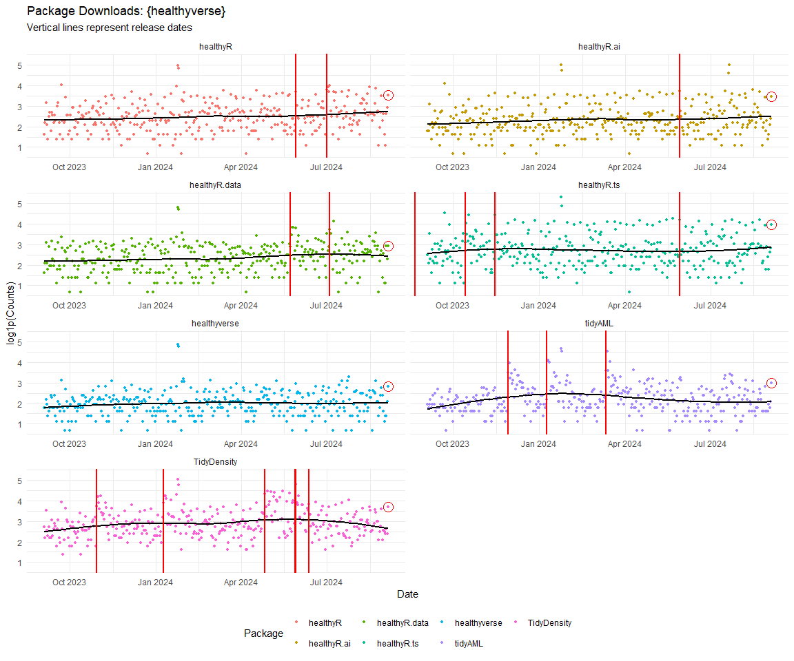
Plots
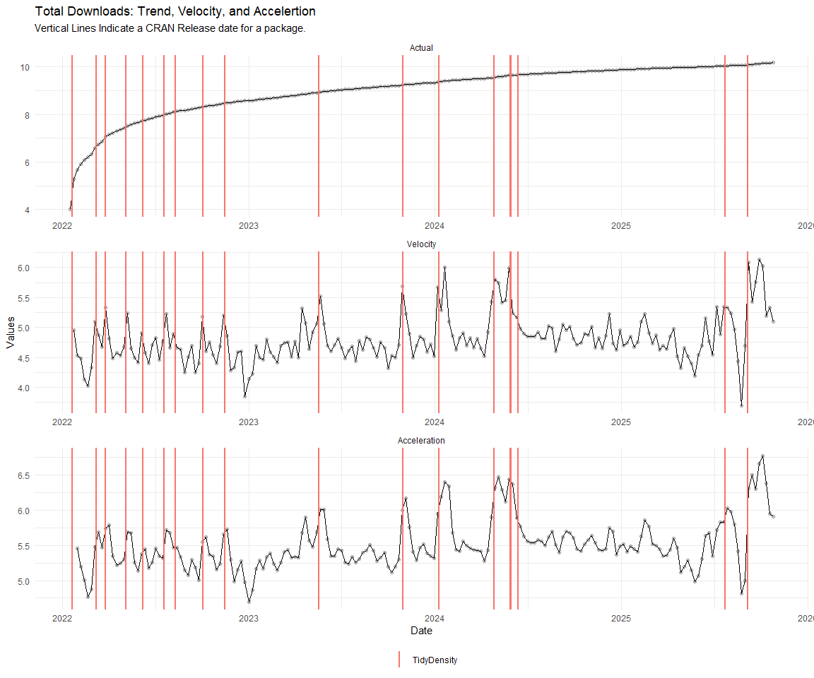
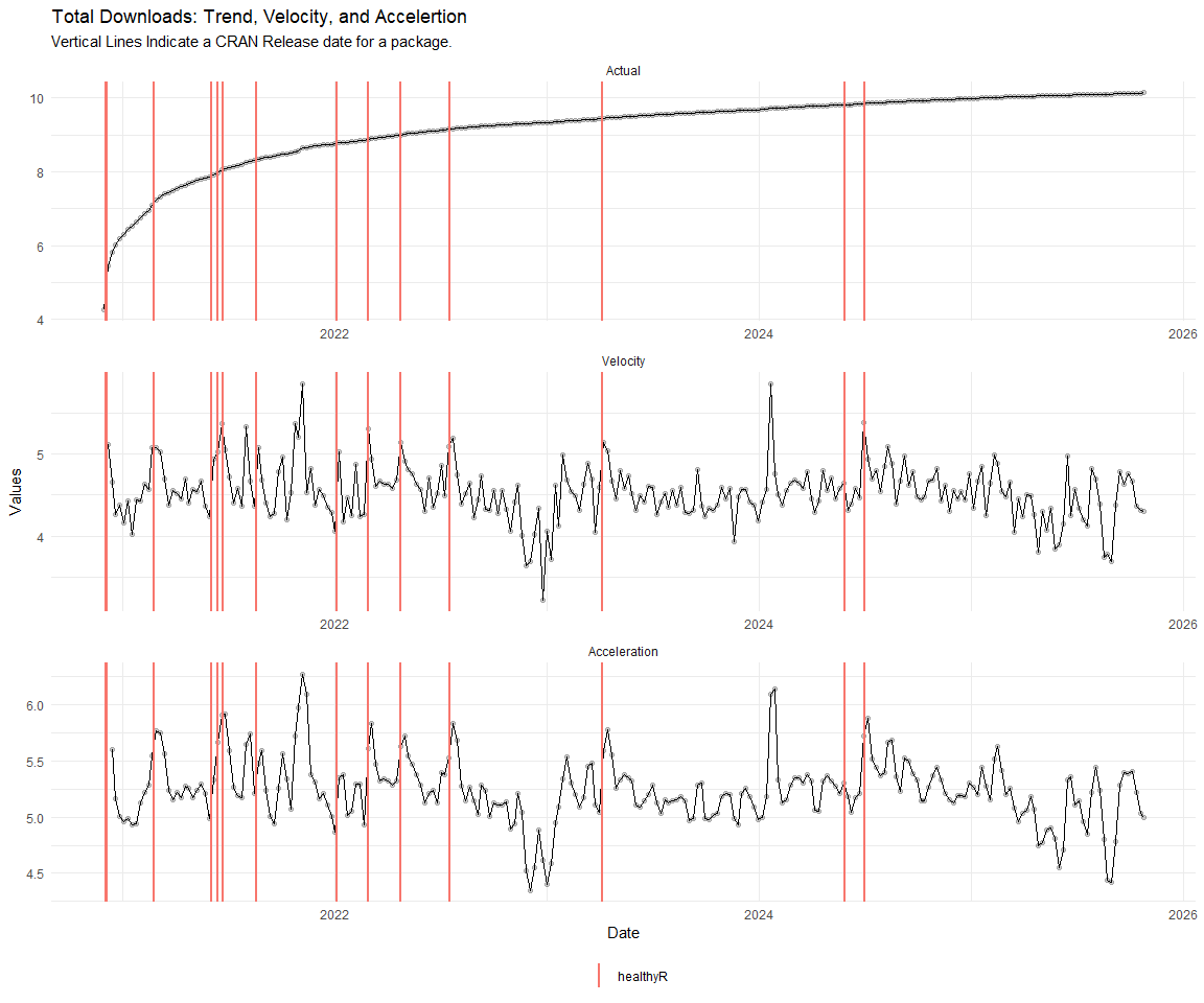
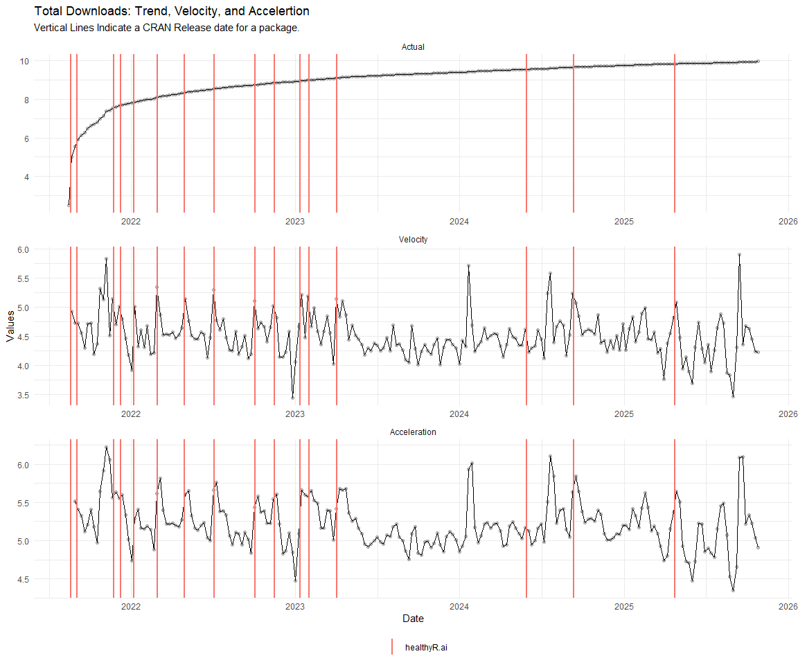
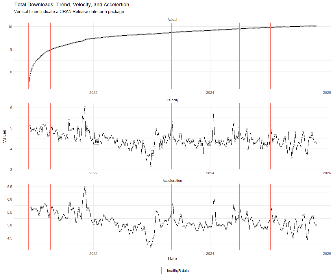
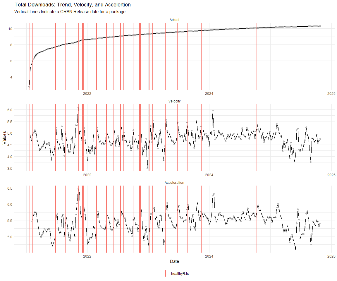
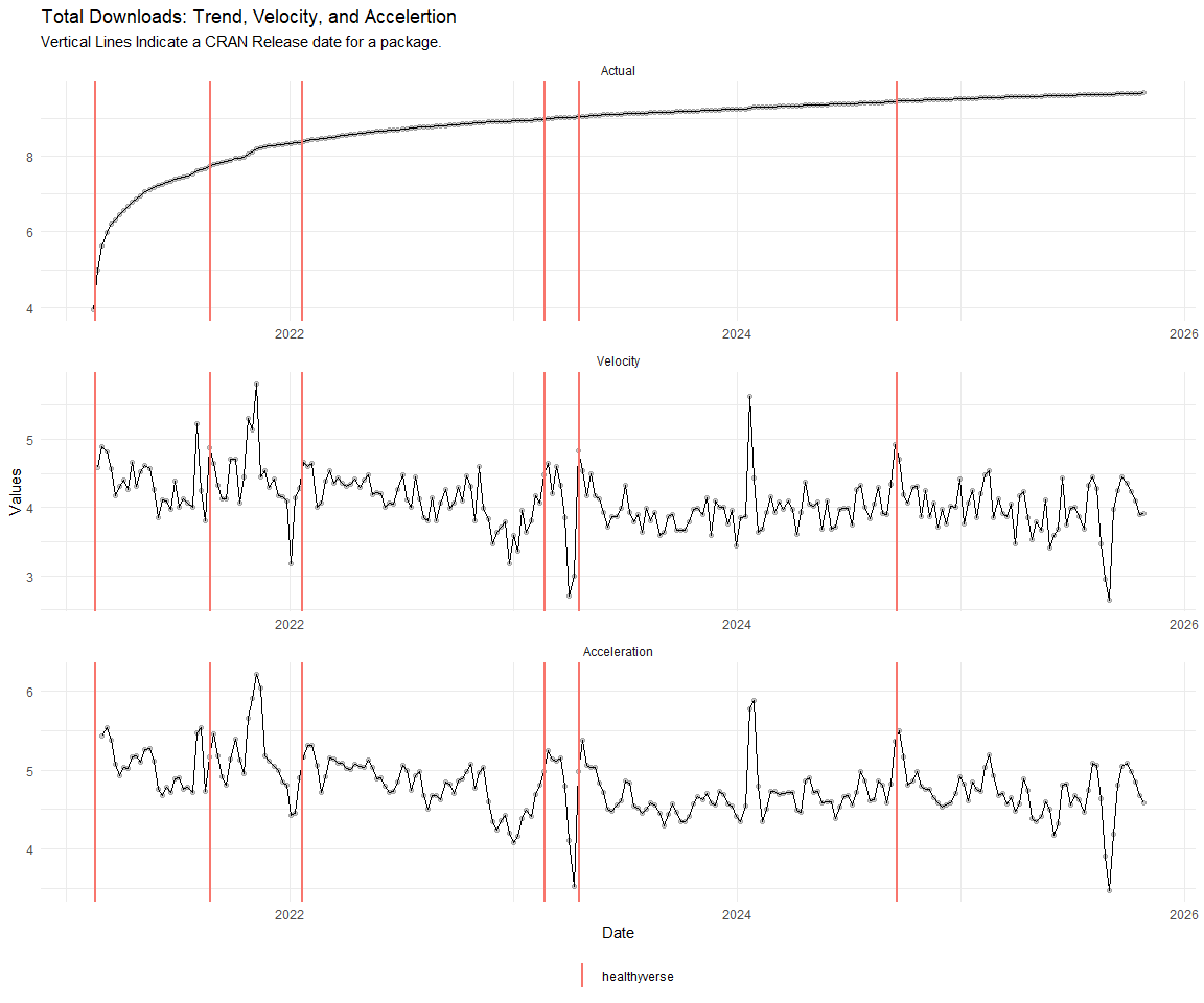
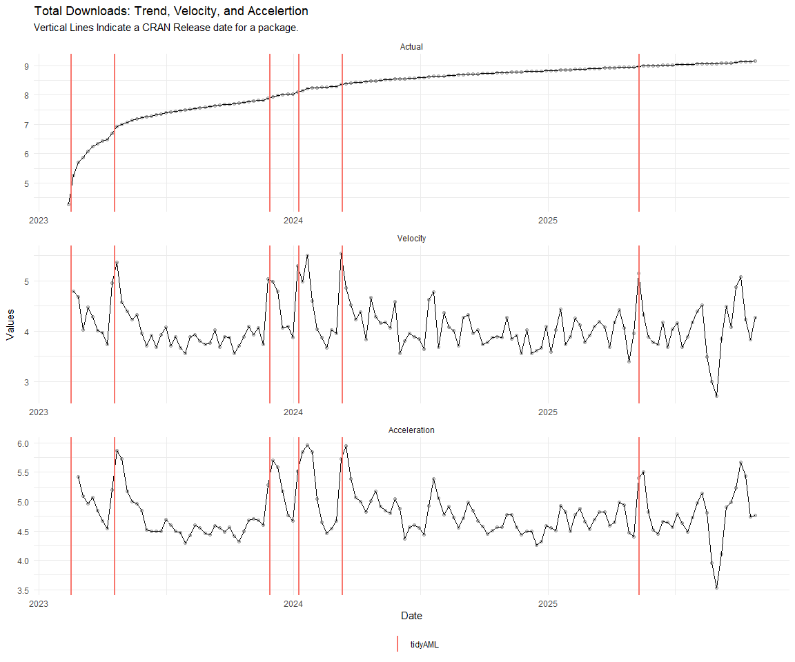
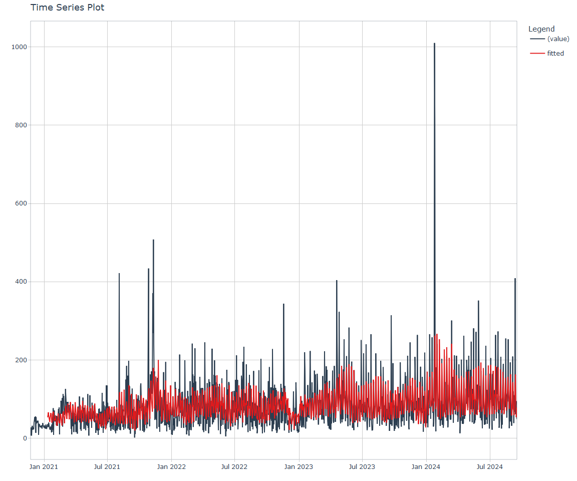
Now lets take a look at a time-series plot of the total daily downloads by package. We will use a log scale and place a vertical line at each version release for each package.
[[1]]
[[2]]
[[3]]
[[4]]
[[5]]
[[6]]
[[7]]
[[8]]
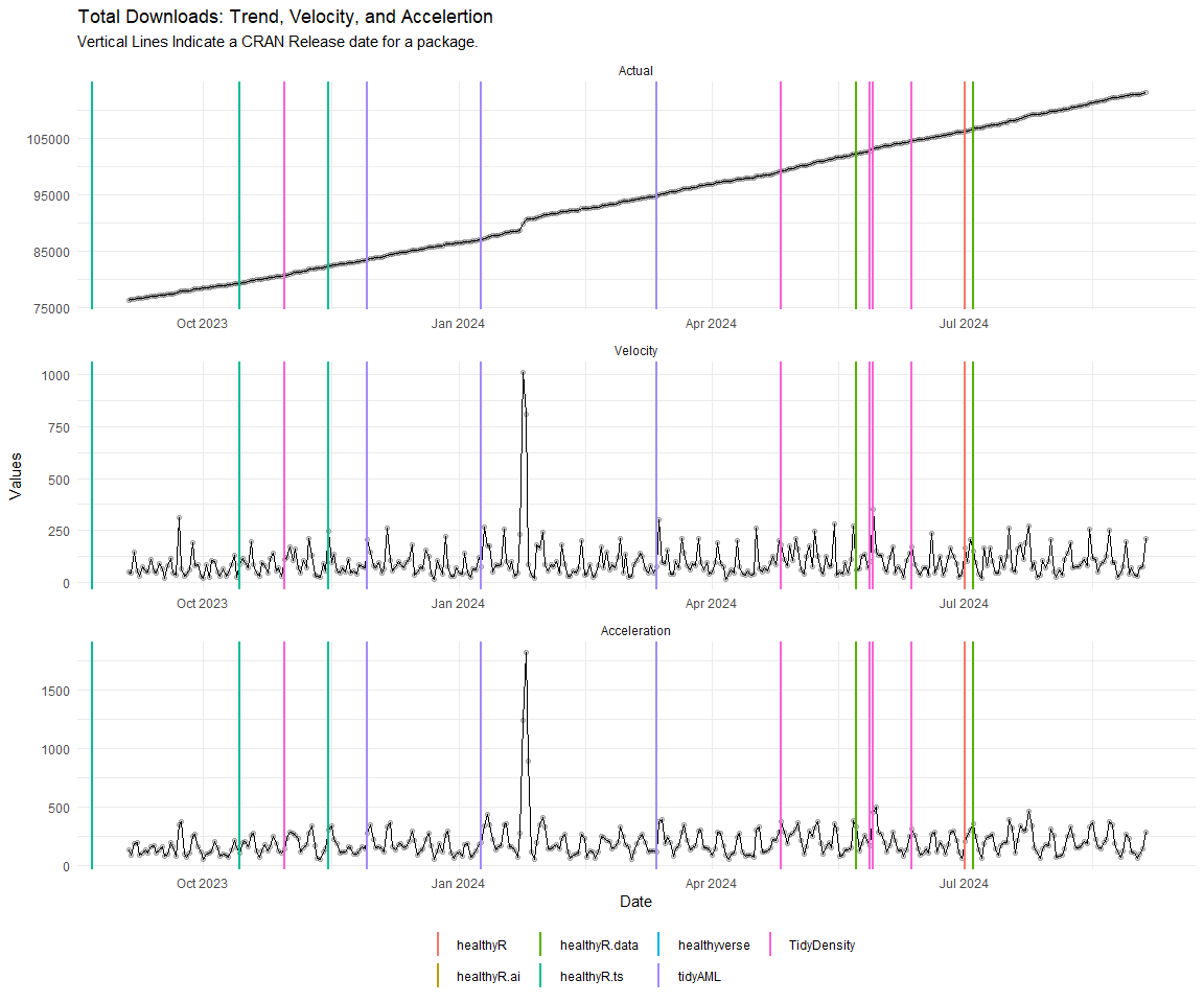
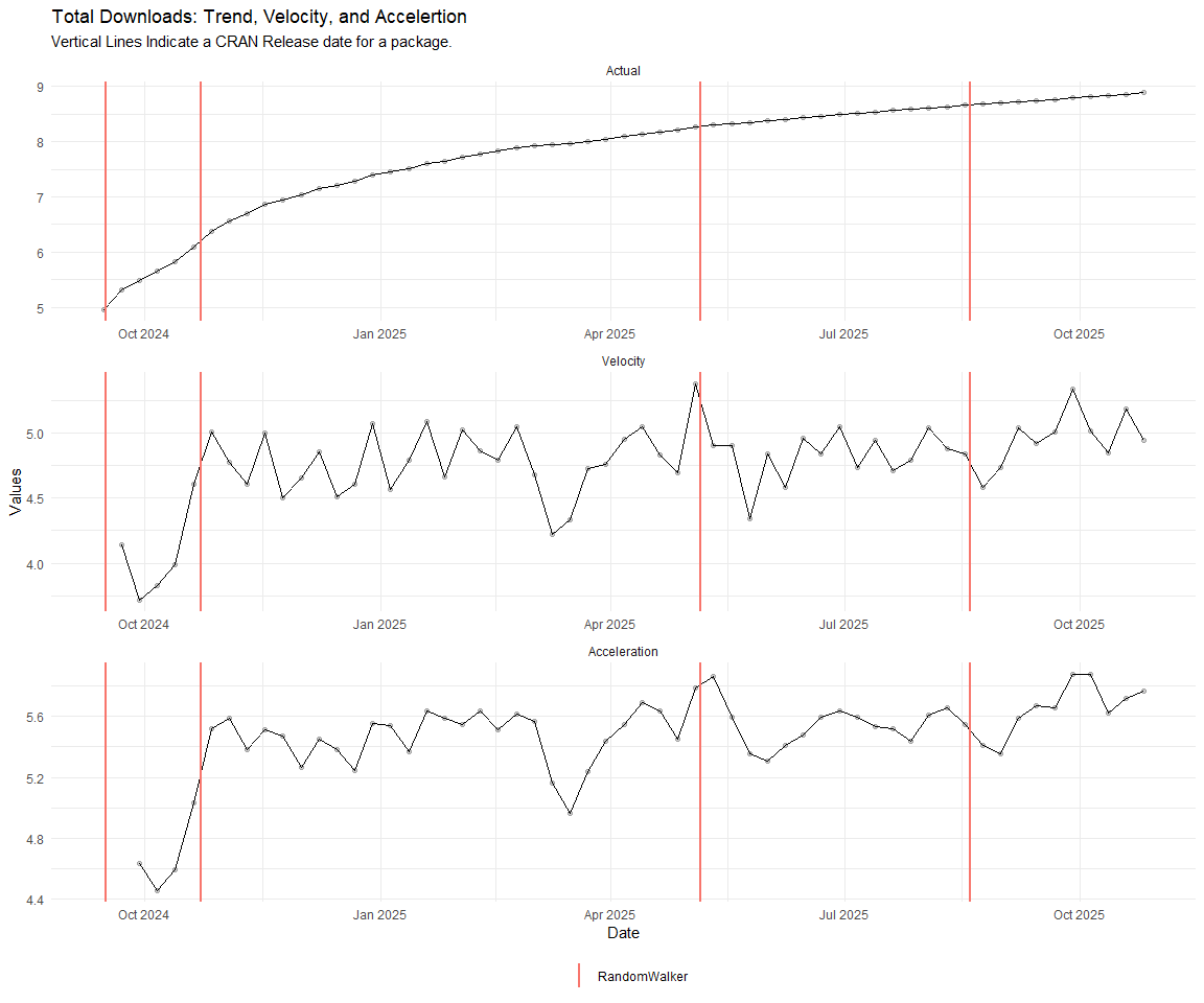
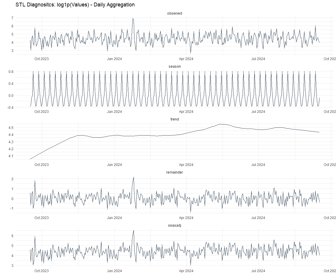
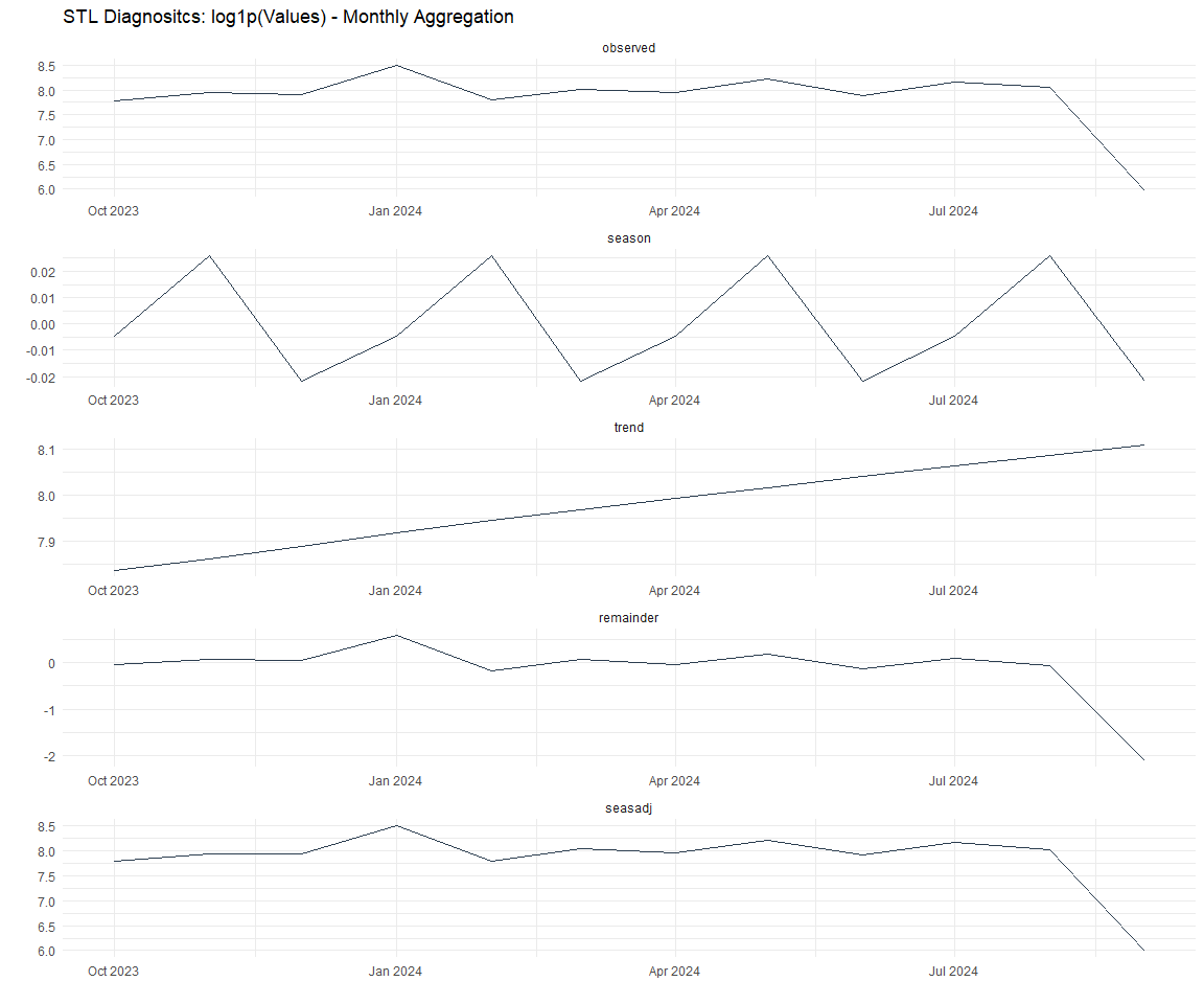
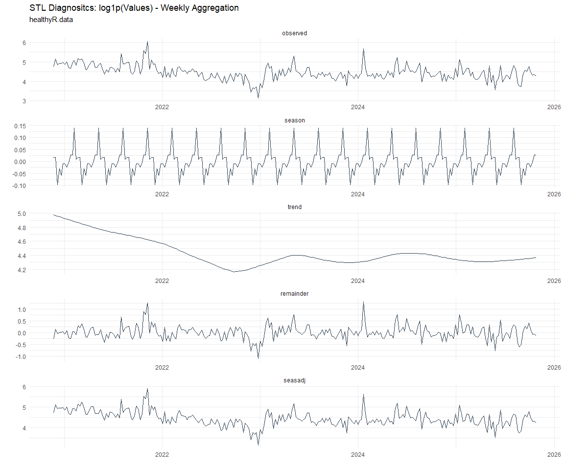
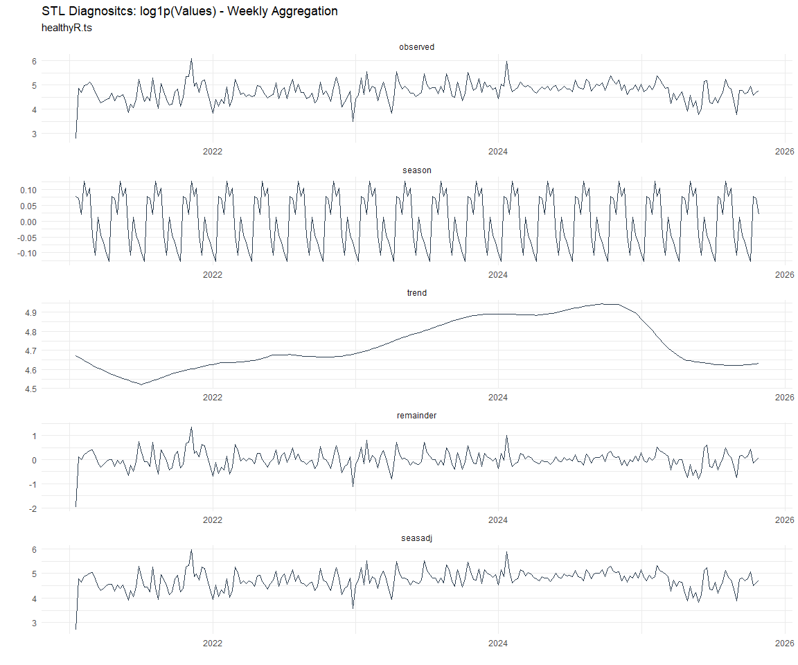
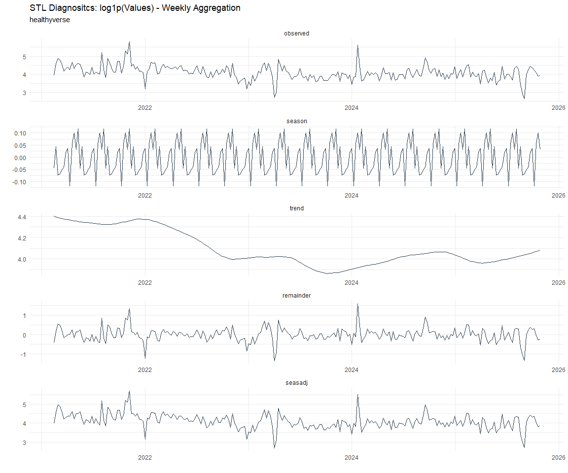
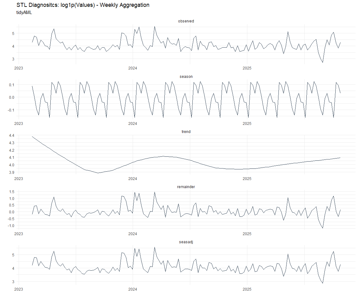
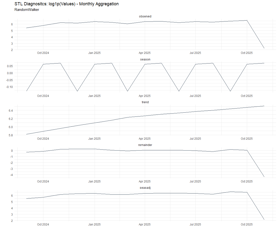
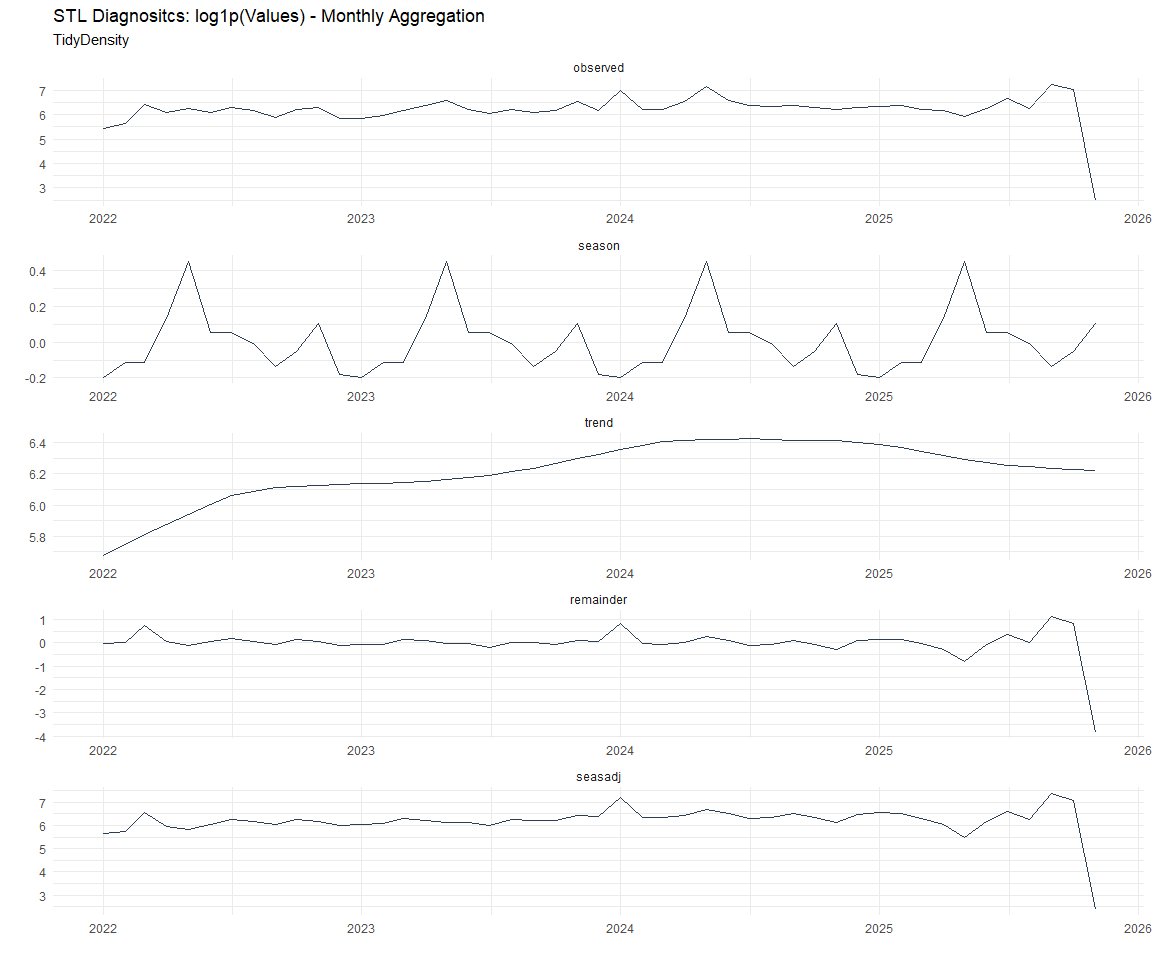
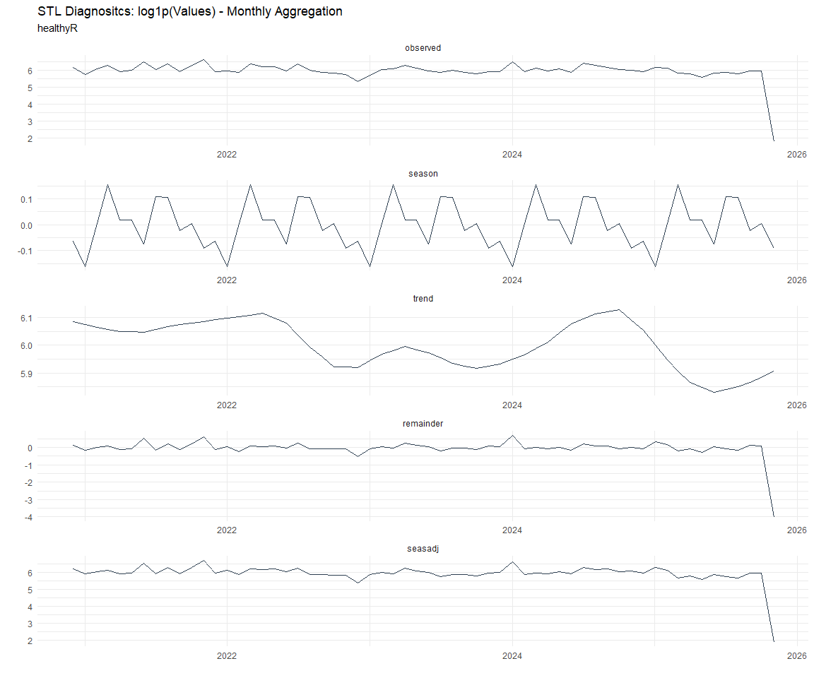
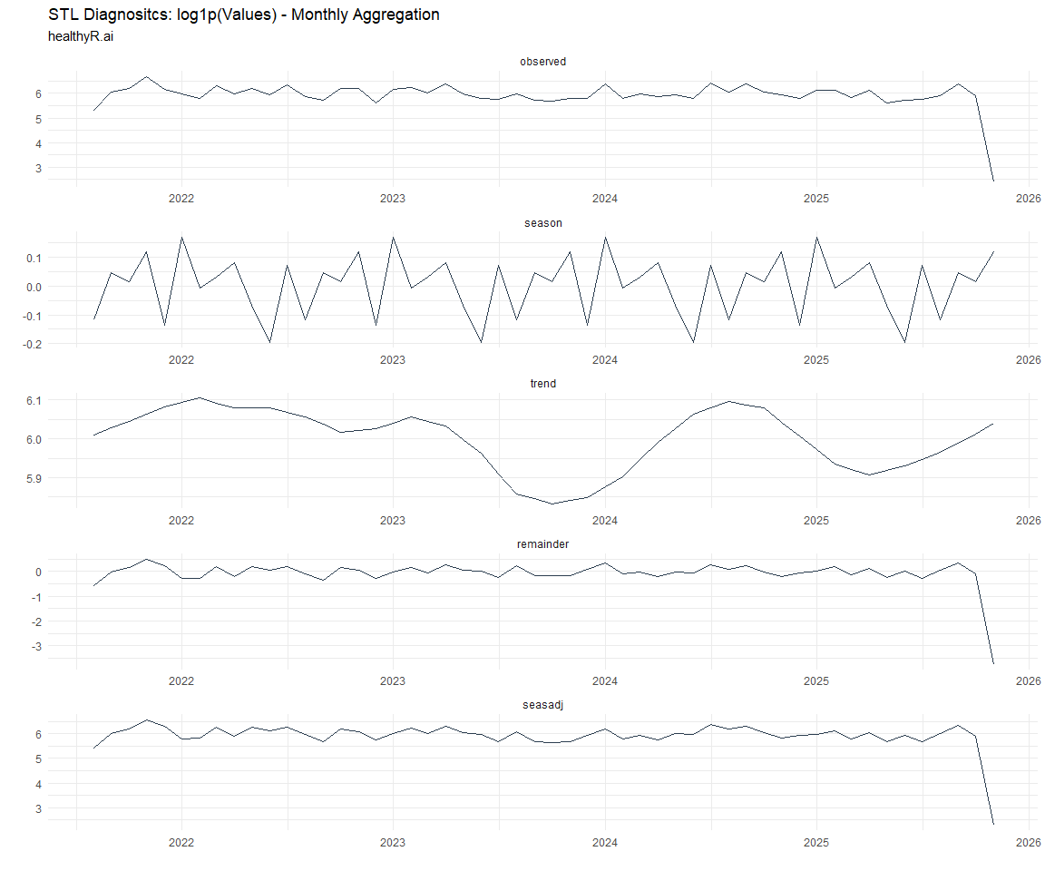
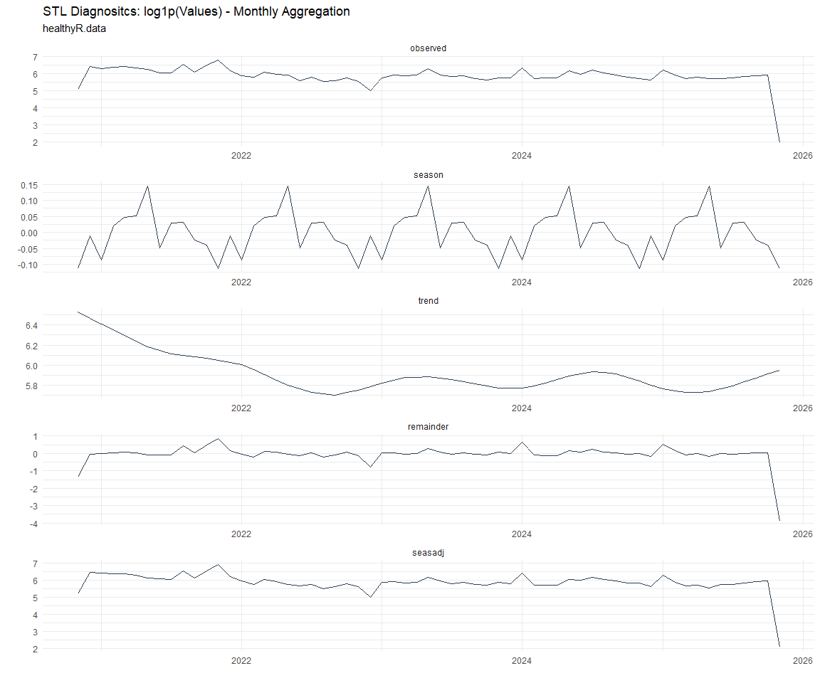
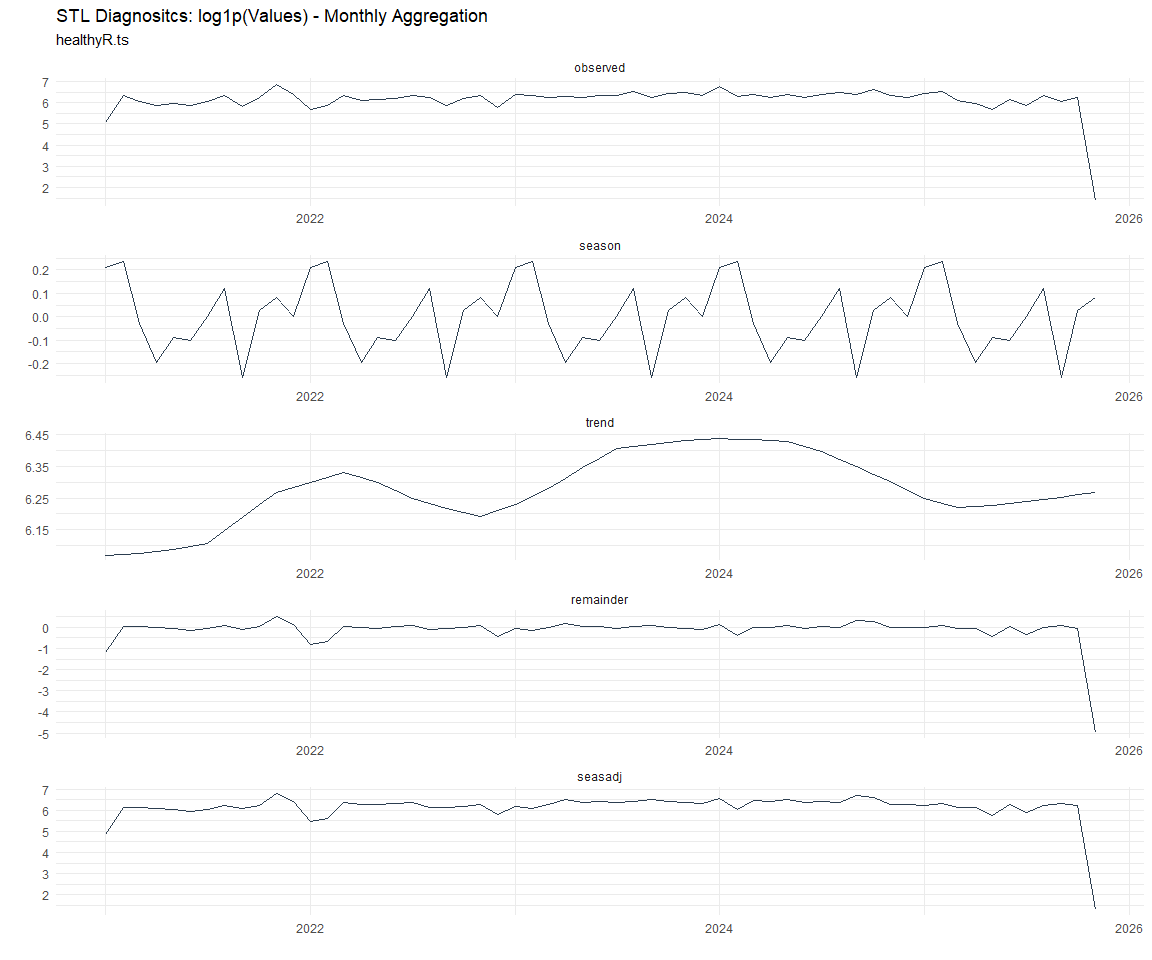
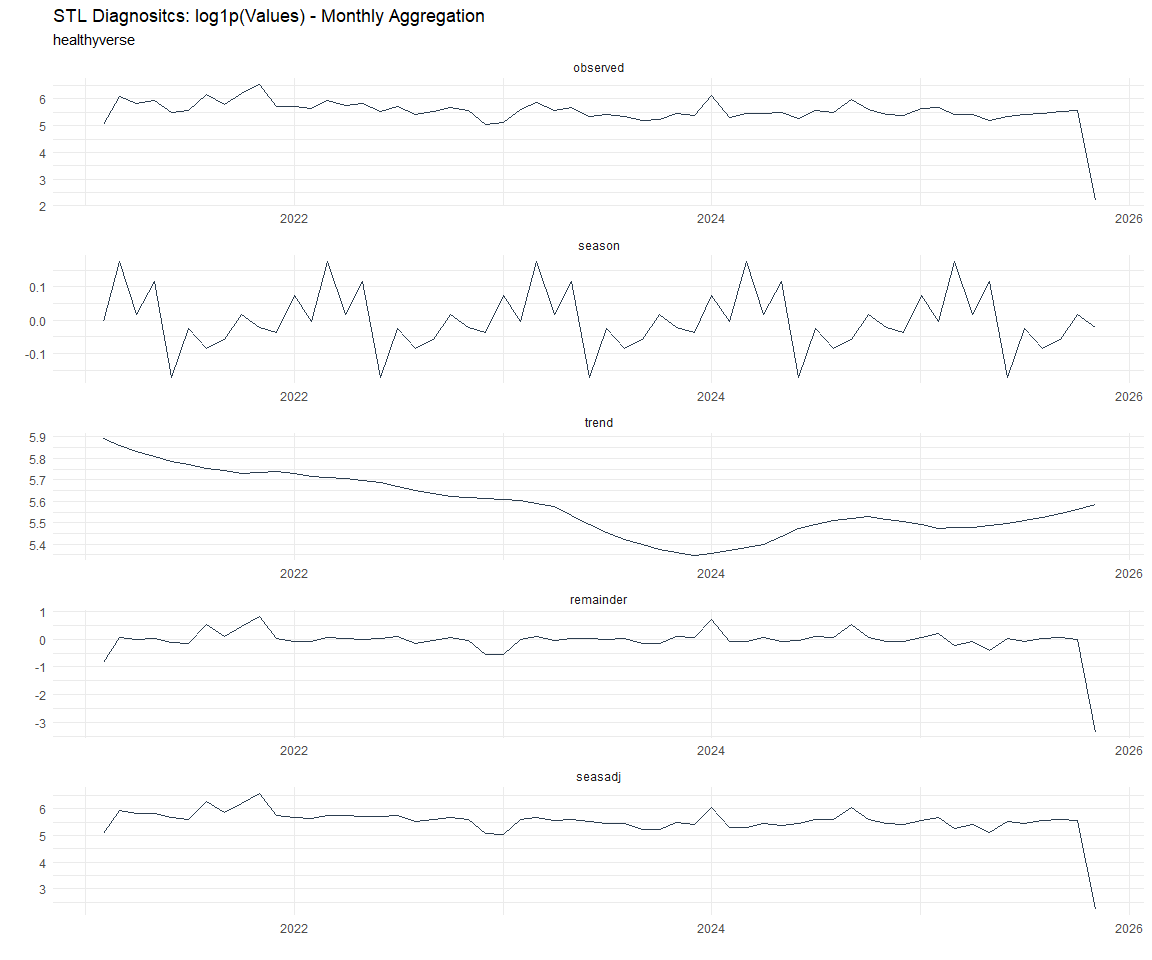
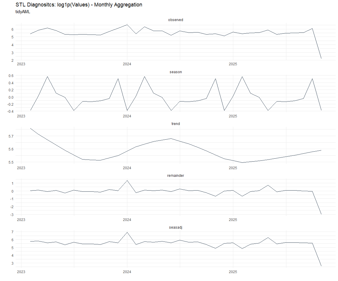
Now lets take a look at some time series decomposition graphs.
[[1]]
[[2]]
[[3]]
[[4]]

[[5]]
[[6]]
[[7]]
[[8]]
[[1]]
[[2]]
[[3]]
[[4]]
[[5]]
[[6]]
[[7]]
[[8]]
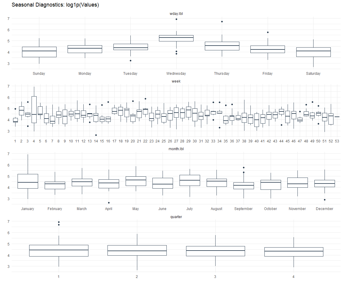
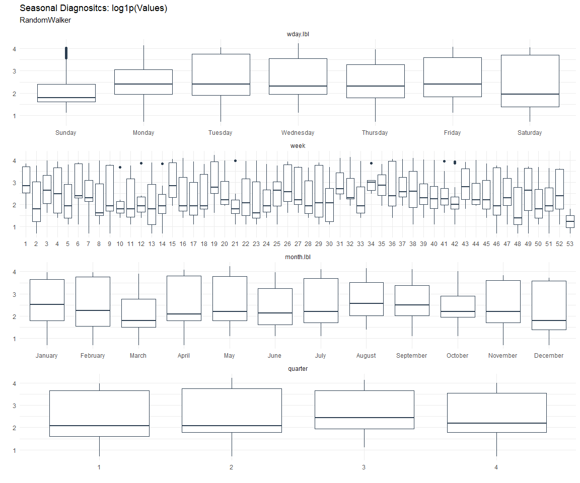
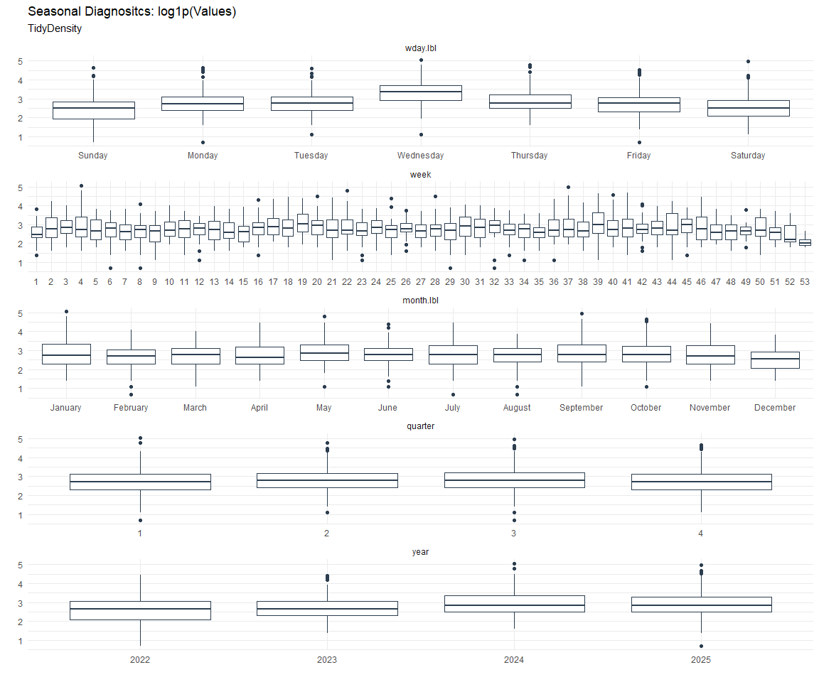
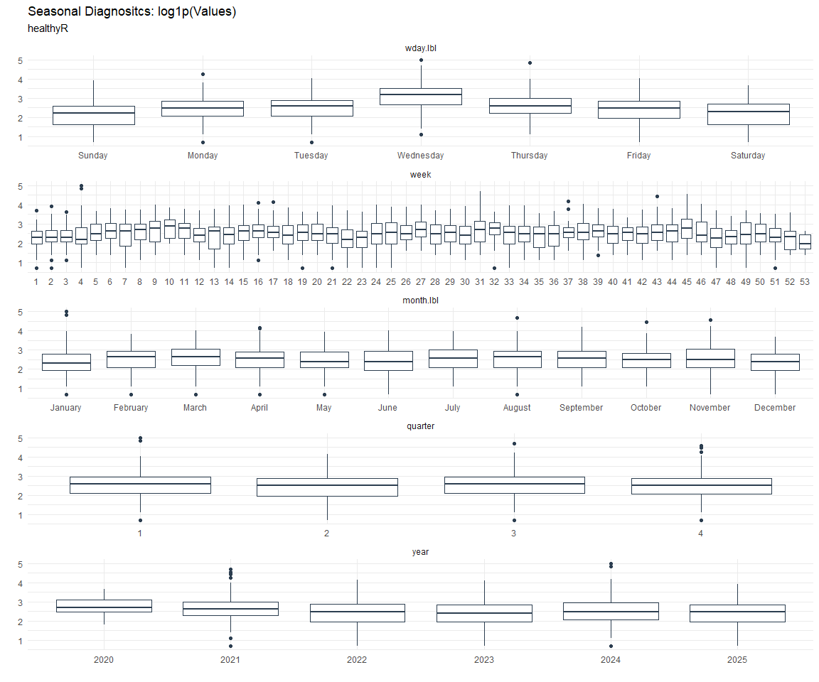
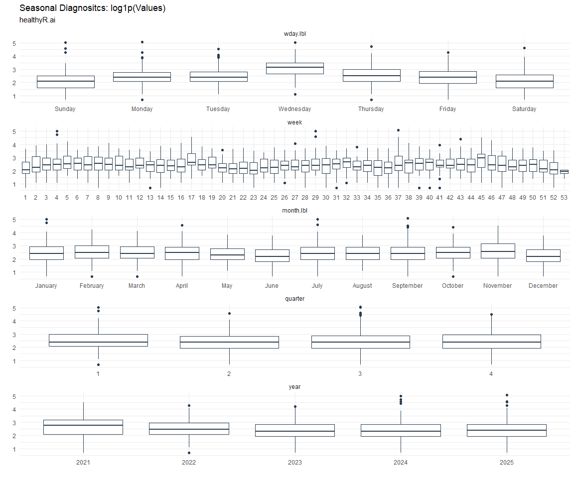
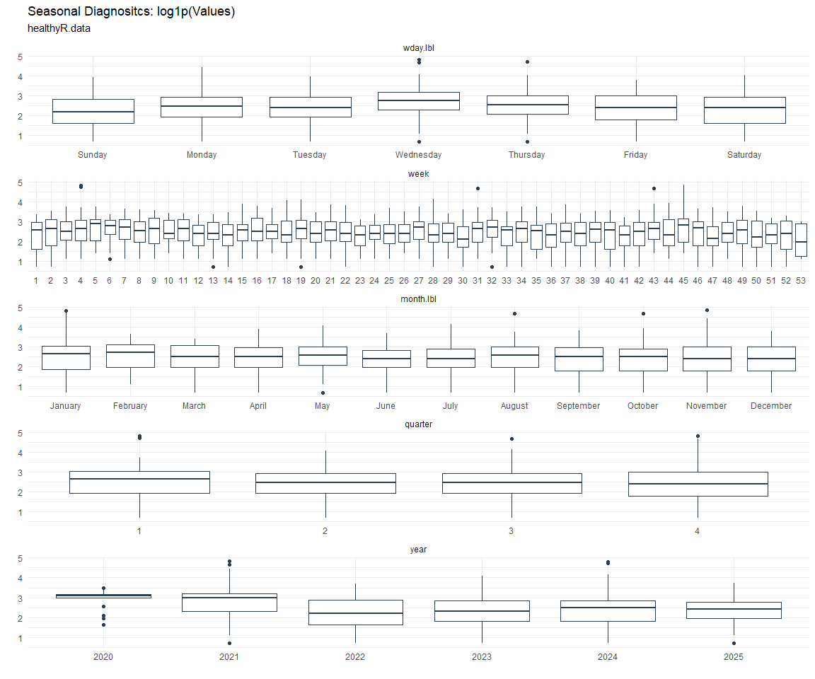
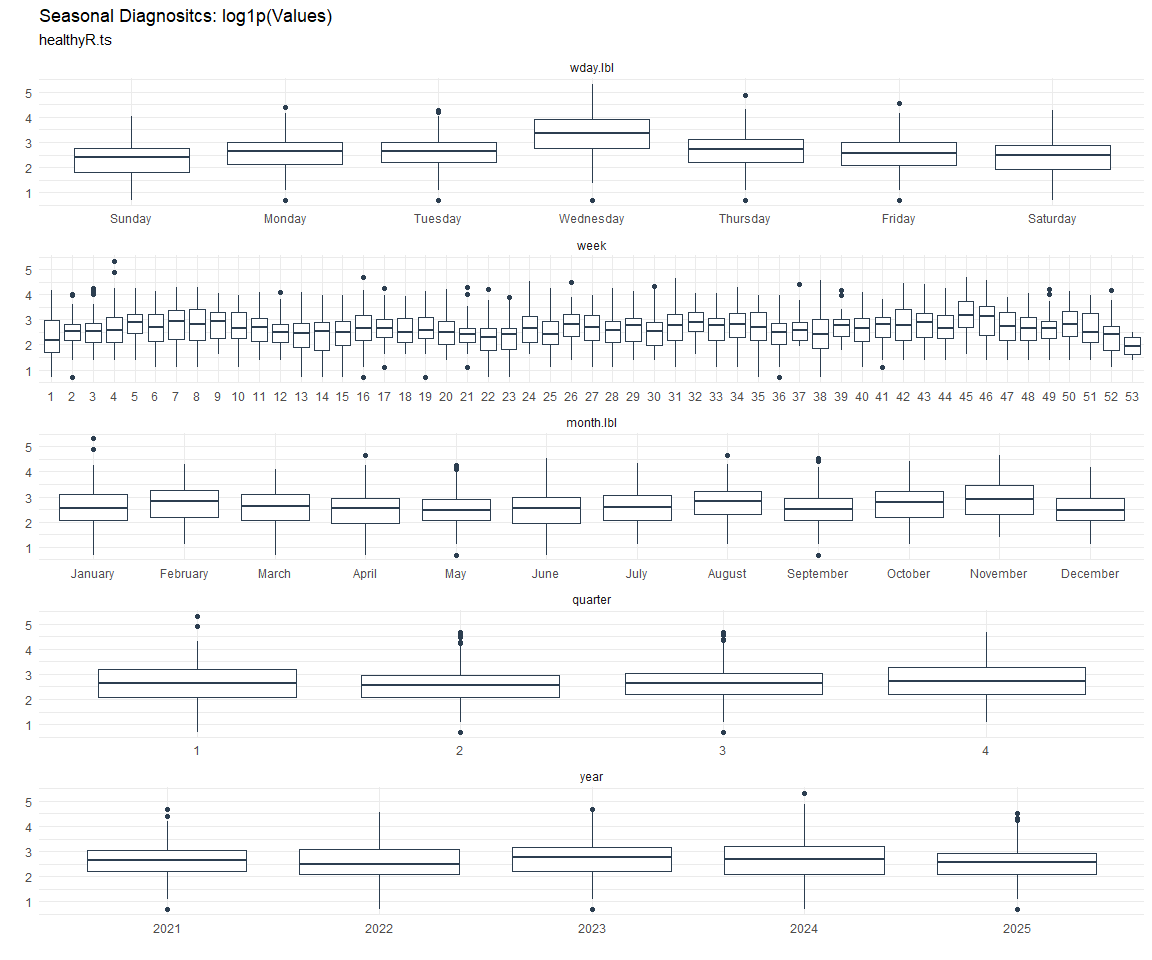
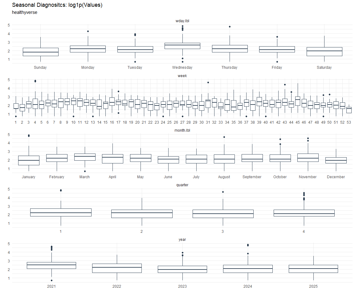
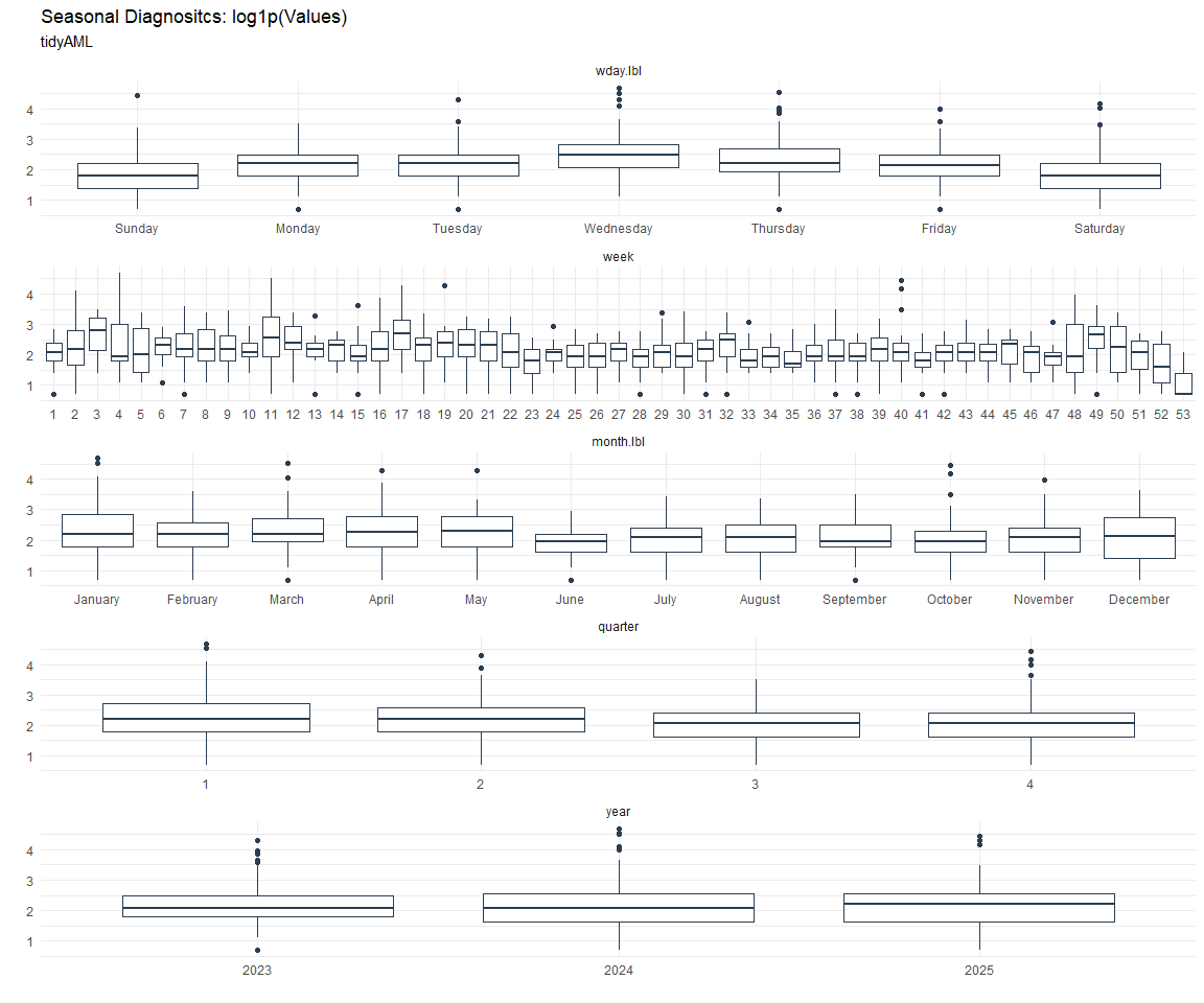
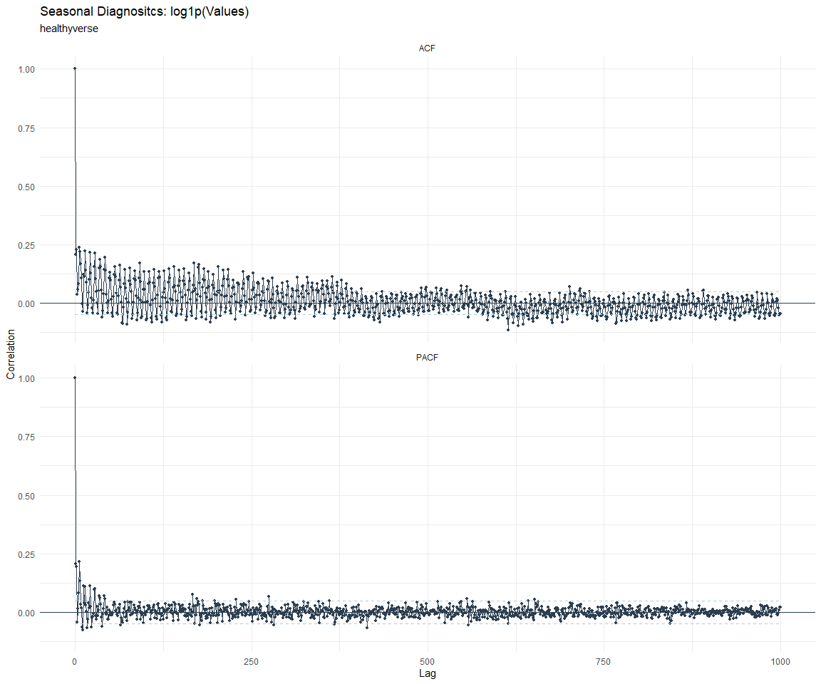
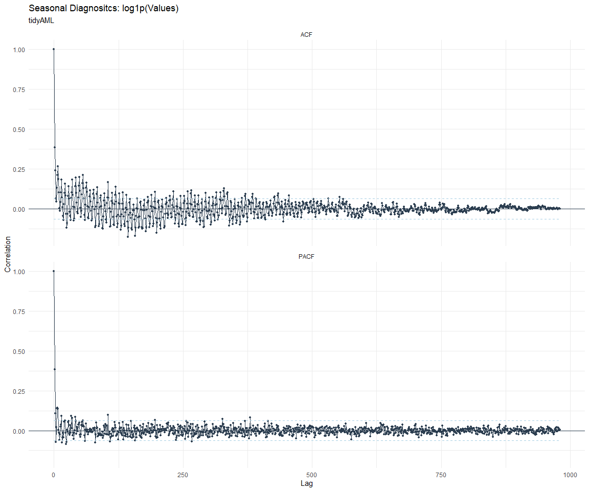
Seasonal Diagnostics:
[[1]]
[[2]]
[[3]]
[[4]]
[[5]]
[[6]]
[[7]]
[[8]]
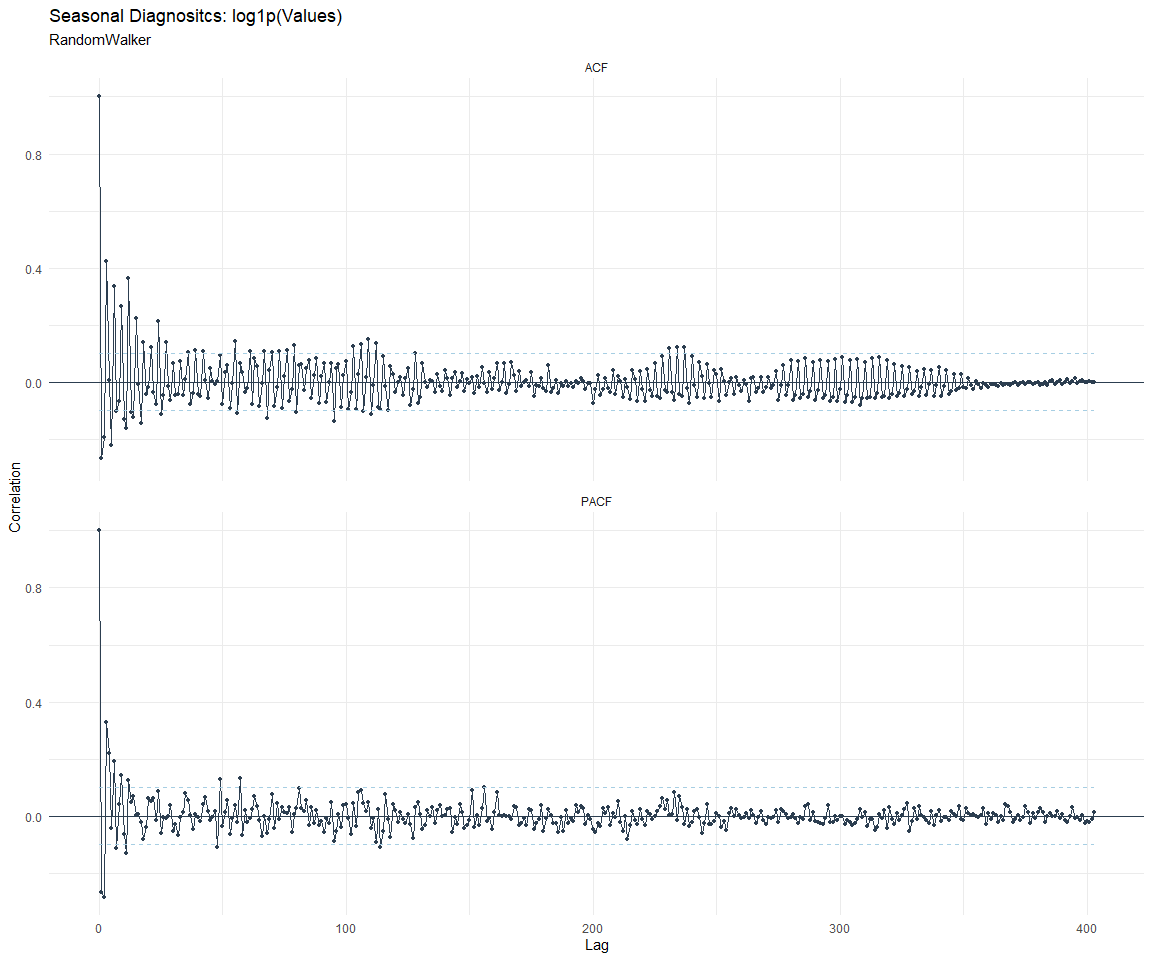
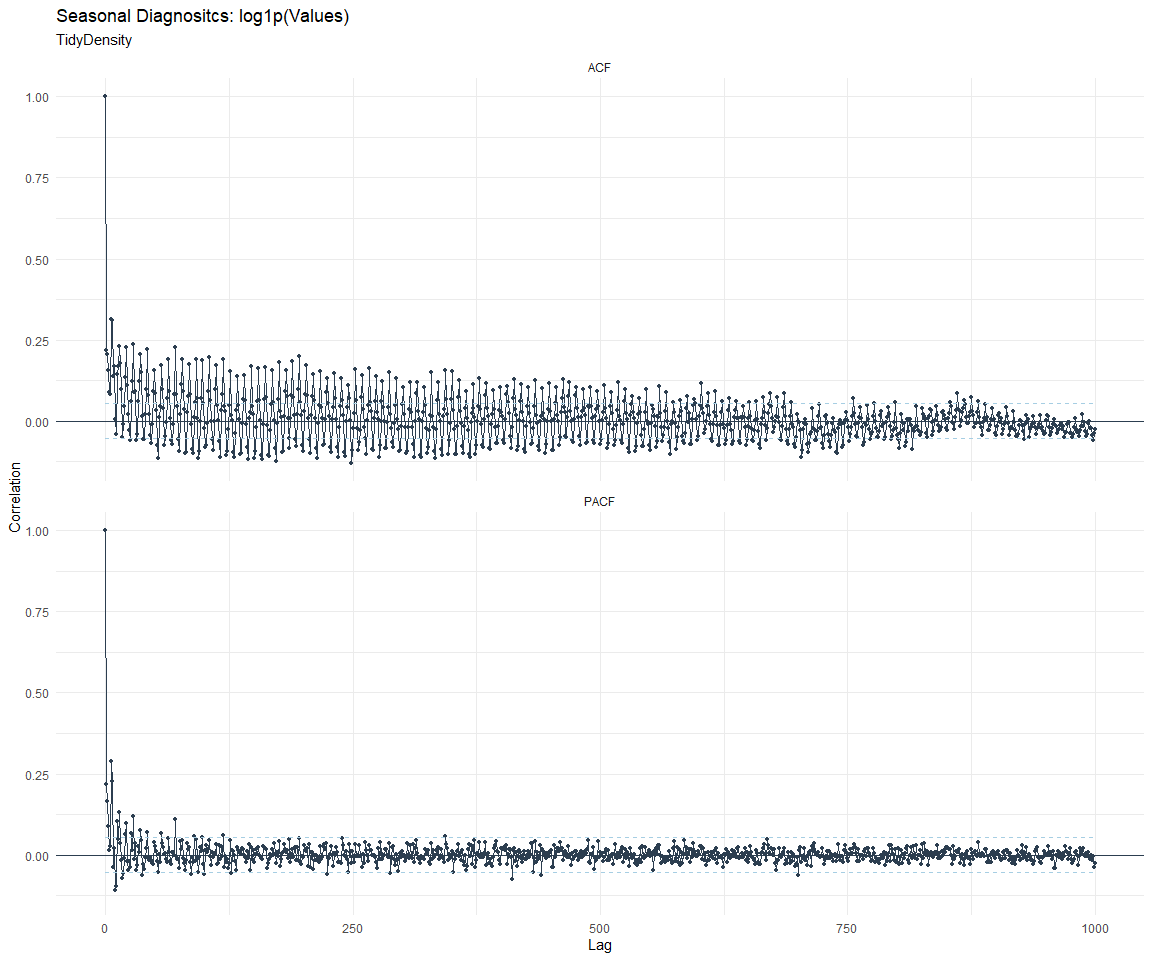
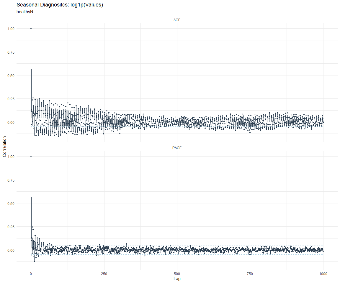
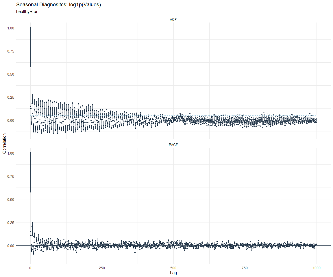
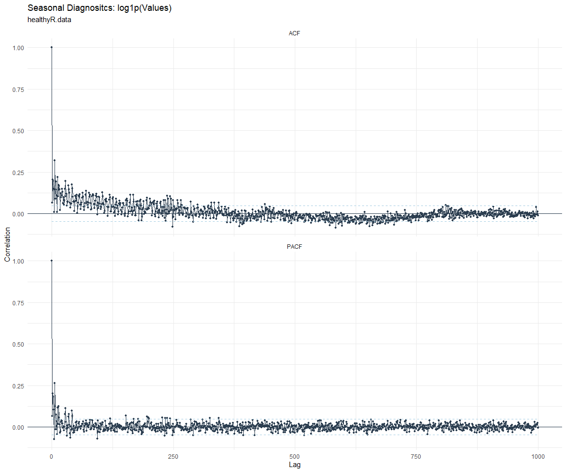
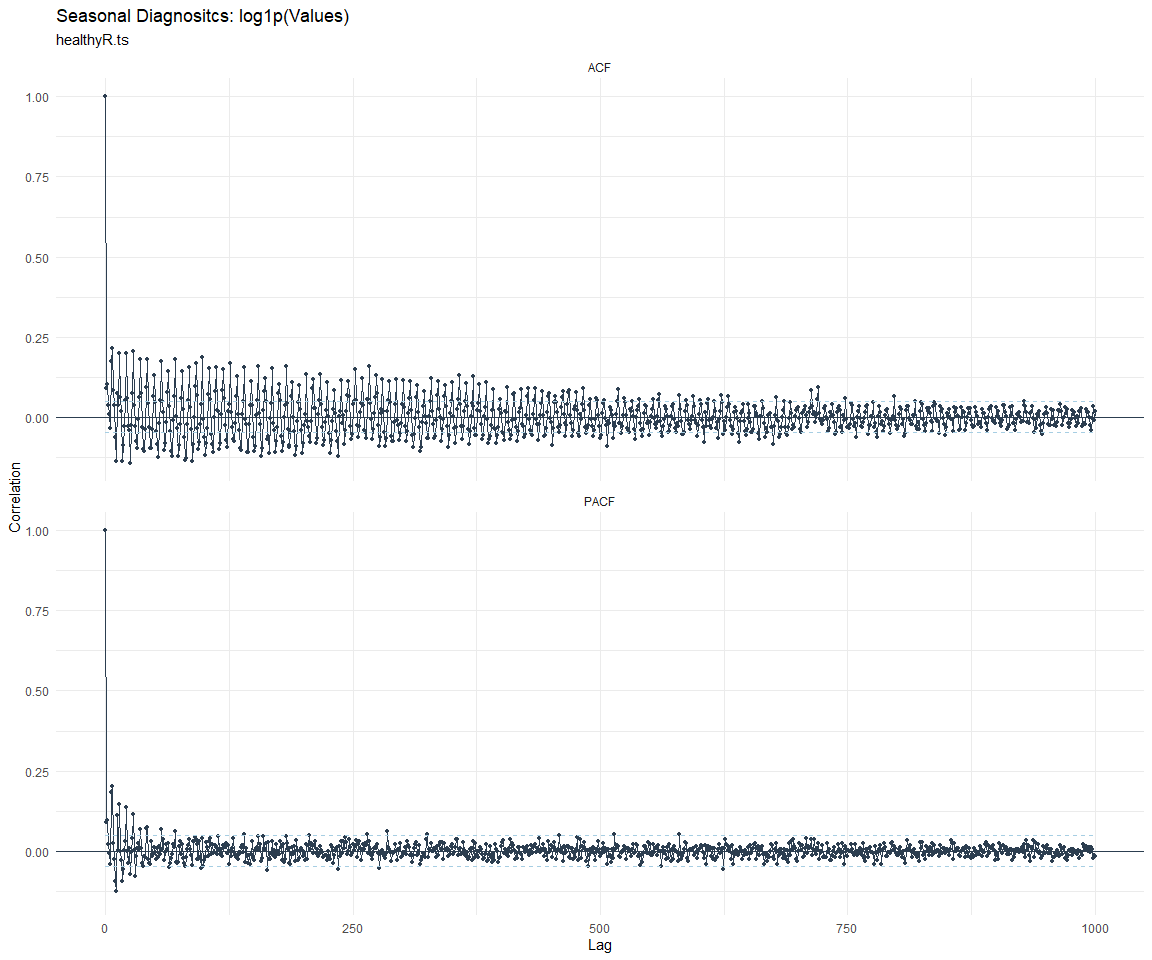
ACF and PACF Diagnostics:
[[1]]
[[2]]
[[3]]
[[4]]
[[5]]
[[6]]
[[7]]
[[8]]
Feature Engineering
Now that we have our basic data and a shot of what it looks like, let’s
add some features to our data which can be very helpful in modeling.
Lets start by making a tibble that is aggregated by the day and
package, as we are going to be interested in forecasting the next 4
weeks or 28 days for each package. First lets get our base data.
Call:
stats::lm(formula = .formula, data = df)

Residuals:
    Min      1Q  Median      3Q     Max
-151.37  -38.11  -11.92   28.32  829.03

Coefficients:
                                                     Estimate Std. Error
(Intercept)                                        -1.650e+02  5.055e+01
date                                                1.044e-02  2.671e-03
lag(value, 1)                                       8.618e-02  2.215e-02
lag(value, 7)                                       6.878e-02  2.273e-02
lag(value, 14)                                      6.448e-02  2.262e-02
lag(value, 21)                                      8.470e-02  2.271e-02
lag(value, 28)                                      8.181e-02  2.267e-02
lag(value, 35)                                      4.129e-02  2.270e-02
lag(value, 42)                                      6.256e-02  2.282e-02
lag(value, 49)                                      7.661e-02  2.274e-02
month(date, label = TRUE).L                        -8.365e+00  4.751e+00
month(date, label = TRUE).Q                        -3.565e-01  4.698e+00
month(date, label = TRUE).C                        -1.611e+01  4.731e+00
month(date, label = TRUE)^4                        -8.209e+00  4.753e+00
month(date, label = TRUE)^5                        -3.899e+00  4.737e+00
month(date, label = TRUE)^6                        -1.888e+00  4.761e+00
month(date, label = TRUE)^7                        -4.293e+00  4.705e+00
month(date, label = TRUE)^8                        -3.164e+00  4.681e+00
month(date, label = TRUE)^9                         2.561e+00  4.697e+00
month(date, label = TRUE)^10                       -2.501e-02  4.707e+00
month(date, label = TRUE)^11                       -3.057e+00  4.685e+00
fourier_vec(date, type = "sin", K = 1, period = 7) -1.084e+01  2.108e+00
fourier_vec(date, type = "cos", K = 1, period = 7)  7.853e+00  2.167e+00
                                                   t value Pr(>|t|)
(Intercept)                                         -3.264 0.001119 **
date                                                 3.909 9.58e-05 ***
lag(value, 1)                                        3.890 0.000103 ***
lag(value, 7)                                        3.026 0.002509 **
lag(value, 14)                                       2.850 0.004412 **
lag(value, 21)                                       3.729 0.000198 ***
lag(value, 28)                                       3.609 0.000315 ***
lag(value, 35)                                       1.819 0.069039 .
lag(value, 42)                                       2.742 0.006165 **
lag(value, 49)                                       3.368 0.000771 ***
month(date, label = TRUE).L                         -1.761 0.078438 .
month(date, label = TRUE).Q                         -0.076 0.939523
month(date, label = TRUE).C                         -3.405 0.000674 ***
month(date, label = TRUE)^4                         -1.727 0.084285 .
month(date, label = TRUE)^5                         -0.823 0.410576
month(date, label = TRUE)^6                         -0.397 0.691724
month(date, label = TRUE)^7                         -0.912 0.361673
month(date, label = TRUE)^8                         -0.676 0.499262
month(date, label = TRUE)^9                          0.545 0.585608
month(date, label = TRUE)^10                        -0.005 0.995762
month(date, label = TRUE)^11                        -0.653 0.514110
fourier_vec(date, type = "sin", K = 1, period = 7)  -5.143 2.97e-07 ***
fourier_vec(date, type = "cos", K = 1, period = 7)   3.624 0.000298 ***
---
Signif. codes:  0 '***' 0.001 '**' 0.01 '*' 0.05 '.' 0.1 ' ' 1

Residual standard error: 60.25 on 1968 degrees of freedom
  (49 observations deleted due to missingness)
Multiple R-squared:  0.2014,    Adjusted R-squared:  0.1925
F-statistic: 22.56 on 22 and 1968 DF,  p-value: < 2.2e-16
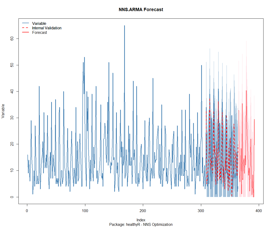
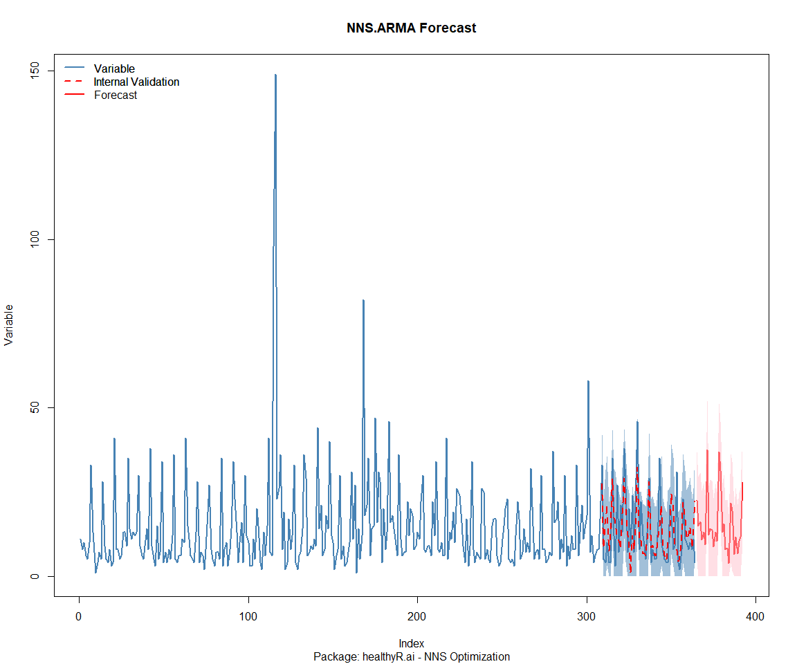
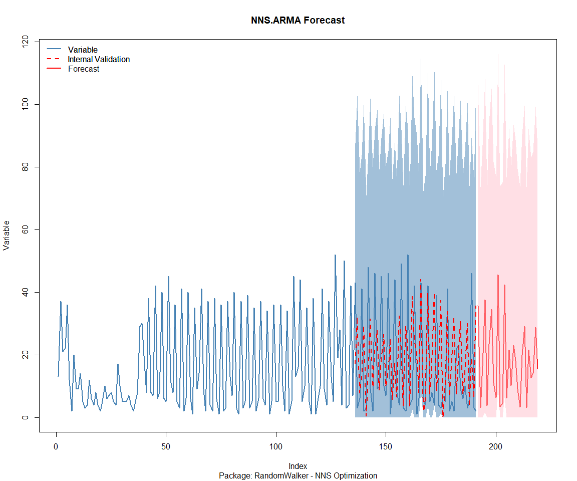
NNS Forecasting
This is something I have been wanting to try for a while. The NNS
package is a great package for forecasting time series data.
library(NNS)

data_list <- base_data |>
    select(package, value) |>
    group_split(package)

data_list |>
    imap(
        \(x, idx) {
            obj <- x
            x <- obj |> pull(value) |> tail(7*52)
            train_set_size <- length(x) - 56
            pkg <- obj |> pluck(1) |> unique()
#            sf <- NNS.seas(x, modulo = 7, plot = FALSE)$periods
            seas <- t(
                sapply(
                    1:25,
                    function(i) c(
                        i,
                        sqrt(
                            mean((
                                NNS.ARMA(x,
                                         h = 28,
                                         training.set = train_set_size,
                                         method = "lin",
                                         seasonal.factor = i,
                                         plot=FALSE
                                         ) - tail(x, 28)) ^ 2)))
                    )
                )
            colnames(seas) <- c("Period", "RMSE")
            sf <- seas[which.min(seas[, 2]), 1]

            cat(paste0("Package: ", pkg, "\n"))
            NNS.ARMA.optim(
                variable = x,
                h = 28,
                training.set = train_set_size,
                #seasonal.factor = seq(12, 60, 7),
                seasonal.factor = sf,
                pred.int = 0.95,
                plot = TRUE
            )
            title(
                sub = paste0("\n",
                             "Package: ", pkg, " - NNS Optimization")
            )
        }
    )
Package: healthyR
[1] "CURRNET METHOD: lin"
[1] "COPY LATEST PARAMETERS DIRECTLY FOR NNS.ARMA() IF ERROR:"
[1] "NNS.ARMA(... method =  'lin' , seasonal.factor =  c( 10 ) ...)"
[1] "CURRENT lin OBJECTIVE FUNCTION = 13.6088368782178"
[1] "BEST method = 'lin' PATH MEMBER = c( 10 )"
[1] "BEST lin OBJECTIVE FUNCTION = 13.6088368782178"
[1] "CURRNET METHOD: nonlin"
[1] "COPY LATEST PARAMETERS DIRECTLY FOR NNS.ARMA() IF ERROR:"
[1] "NNS.ARMA(... method =  'nonlin' , seasonal.factor =  c( 10 ) ...)"
[1] "CURRENT nonlin OBJECTIVE FUNCTION = 8.77778562014289"
[1] "BEST method = 'nonlin' PATH MEMBER = c( 10 )"
[1] "BEST nonlin OBJECTIVE FUNCTION = 8.77778562014289"
[1] "CURRNET METHOD: both"
[1] "COPY LATEST PARAMETERS DIRECTLY FOR NNS.ARMA() IF ERROR:"
[1] "NNS.ARMA(... method =  'both' , seasonal.factor =  c( 10 ) ...)"
[1] "CURRENT both OBJECTIVE FUNCTION = 10.958990736726"
[1] "BEST method = 'both' PATH MEMBER = c( 10 )"
[1] "BEST both OBJECTIVE FUNCTION = 10.958990736726"
Package: healthyR.ai
[1] "CURRNET METHOD: lin"
[1] "COPY LATEST PARAMETERS DIRECTLY FOR NNS.ARMA() IF ERROR:"
[1] "NNS.ARMA(... method =  'lin' , seasonal.factor =  c( 16 ) ...)"
[1] "CURRENT lin OBJECTIVE FUNCTION = 12.2025538251828"
[1] "BEST method = 'lin' PATH MEMBER = c( 16 )"
[1] "BEST lin OBJECTIVE FUNCTION = 12.2025538251828"
[1] "CURRNET METHOD: nonlin"
[1] "COPY LATEST PARAMETERS DIRECTLY FOR NNS.ARMA() IF ERROR:"
[1] "NNS.ARMA(... method =  'nonlin' , seasonal.factor =  c( 16 ) ...)"
[1] "CURRENT nonlin OBJECTIVE FUNCTION = 10.6759787987636"
[1] "BEST method = 'nonlin' PATH MEMBER = c( 16 )"
[1] "BEST nonlin OBJECTIVE FUNCTION = 10.6759787987636"
[1] "CURRNET METHOD: both"
[1] "COPY LATEST PARAMETERS DIRECTLY FOR NNS.ARMA() IF ERROR:"
[1] "NNS.ARMA(... method =  'both' , seasonal.factor =  c( 16 ) ...)"
[1] "CURRENT both OBJECTIVE FUNCTION = 10.6880030492137"
[1] "BEST method = 'both' PATH MEMBER = c( 16 )"
[1] "BEST both OBJECTIVE FUNCTION = 10.6880030492137"
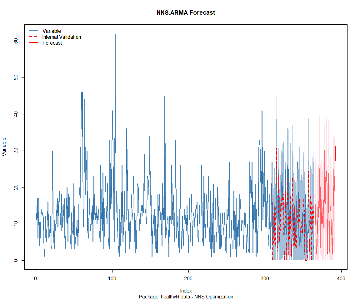
Package: healthyR.data
[1] "CURRNET METHOD: lin"
[1] "COPY LATEST PARAMETERS DIRECTLY FOR NNS.ARMA() IF ERROR:"
[1] "NNS.ARMA(... method =  'lin' , seasonal.factor =  c( 22 ) ...)"
[1] "CURRENT lin OBJECTIVE FUNCTION = 5.87498129992533"
[1] "BEST method = 'lin' PATH MEMBER = c( 22 )"
[1] "BEST lin OBJECTIVE FUNCTION = 5.87498129992533"
[1] "CURRNET METHOD: nonlin"
[1] "COPY LATEST PARAMETERS DIRECTLY FOR NNS.ARMA() IF ERROR:"
[1] "NNS.ARMA(... method =  'nonlin' , seasonal.factor =  c( 22 ) ...)"
[1] "CURRENT nonlin OBJECTIVE FUNCTION = 6.37890072305874"
[1] "BEST method = 'nonlin' PATH MEMBER = c( 22 )"
[1] "BEST nonlin OBJECTIVE FUNCTION = 6.37890072305874"
[1] "CURRNET METHOD: both"
[1] "COPY LATEST PARAMETERS DIRECTLY FOR NNS.ARMA() IF ERROR:"
[1] "NNS.ARMA(... method =  'both' , seasonal.factor =  c( 22 ) ...)"
[1] "CURRENT both OBJECTIVE FUNCTION = 4.71324066817254"
[1] "BEST method = 'both' PATH MEMBER = c( 22 )"
[1] "BEST both OBJECTIVE FUNCTION = 4.71324066817254"
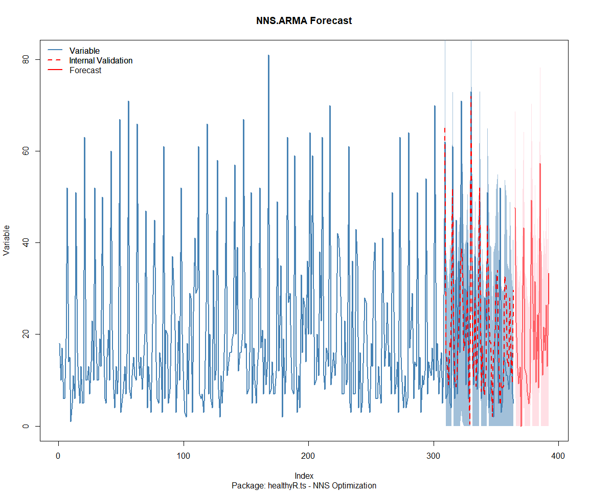
Package: healthyR.ts
[1] "CURRNET METHOD: lin"
[1] "COPY LATEST PARAMETERS DIRECTLY FOR NNS.ARMA() IF ERROR:"
[1] "NNS.ARMA(... method =  'lin' , seasonal.factor =  c( 10 ) ...)"
[1] "CURRENT lin OBJECTIVE FUNCTION = 30.1472229638499"
[1] "BEST method = 'lin' PATH MEMBER = c( 10 )"
[1] "BEST lin OBJECTIVE FUNCTION = 30.1472229638499"
[1] "CURRNET METHOD: nonlin"
[1] "COPY LATEST PARAMETERS DIRECTLY FOR NNS.ARMA() IF ERROR:"
[1] "NNS.ARMA(... method =  'nonlin' , seasonal.factor =  c( 10 ) ...)"
[1] "CURRENT nonlin OBJECTIVE FUNCTION = 22.5471820139151"
[1] "BEST method = 'nonlin' PATH MEMBER = c( 10 )"
[1] "BEST nonlin OBJECTIVE FUNCTION = 22.5471820139151"
[1] "CURRNET METHOD: both"
[1] "COPY LATEST PARAMETERS DIRECTLY FOR NNS.ARMA() IF ERROR:"
[1] "NNS.ARMA(... method =  'both' , seasonal.factor =  c( 10 ) ...)"
[1] "CURRENT both OBJECTIVE FUNCTION = 29.125307701216"
[1] "BEST method = 'both' PATH MEMBER = c( 10 )"
[1] "BEST both OBJECTIVE FUNCTION = 29.125307701216"
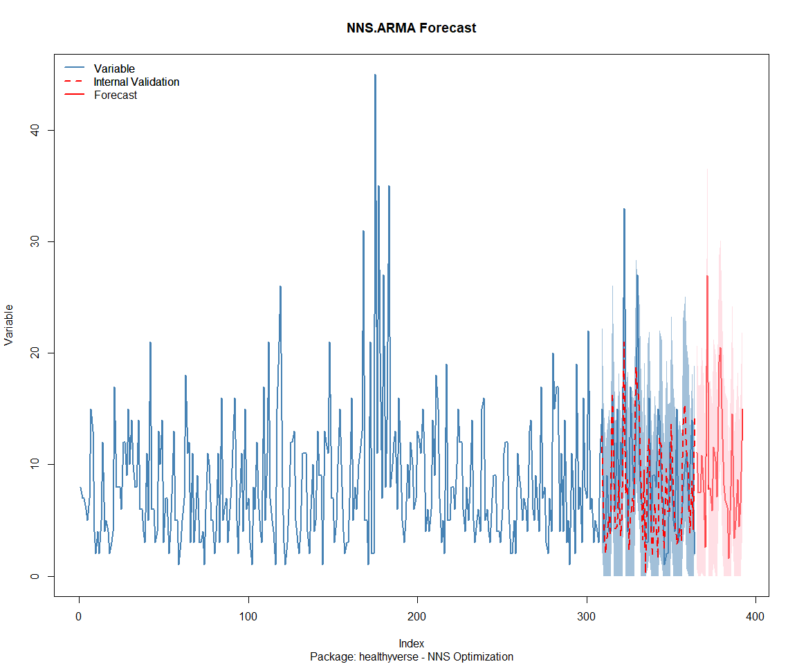
Package: healthyverse
[1] "CURRNET METHOD: lin"
[1] "COPY LATEST PARAMETERS DIRECTLY FOR NNS.ARMA() IF ERROR:"
[1] "NNS.ARMA(... method =  'lin' , seasonal.factor =  c( 11 ) ...)"
[1] "CURRENT lin OBJECTIVE FUNCTION = 8.16326861336829"
[1] "BEST method = 'lin' PATH MEMBER = c( 11 )"
[1] "BEST lin OBJECTIVE FUNCTION = 8.16326861336829"
[1] "CURRNET METHOD: nonlin"
[1] "COPY LATEST PARAMETERS DIRECTLY FOR NNS.ARMA() IF ERROR:"
[1] "NNS.ARMA(... method =  'nonlin' , seasonal.factor =  c( 11 ) ...)"
[1] "CURRENT nonlin OBJECTIVE FUNCTION = 7.6261351606125"
[1] "BEST method = 'nonlin' PATH MEMBER = c( 11 )"
[1] "BEST nonlin OBJECTIVE FUNCTION = 7.6261351606125"
[1] "CURRNET METHOD: both"
[1] "COPY LATEST PARAMETERS DIRECTLY FOR NNS.ARMA() IF ERROR:"
[1] "NNS.ARMA(... method =  'both' , seasonal.factor =  c( 11 ) ...)"
[1] "CURRENT both OBJECTIVE FUNCTION = 7.90811984083281"
[1] "BEST method = 'both' PATH MEMBER = c( 11 )"
[1] "BEST both OBJECTIVE FUNCTION = 7.90811984083281"
Package: RandomWalker
[1] "CURRNET METHOD: lin"
[1] "COPY LATEST PARAMETERS DIRECTLY FOR NNS.ARMA() IF ERROR:"
[1] "NNS.ARMA(... method =  'lin' , seasonal.factor =  c( 4 ) ...)"
[1] "CURRENT lin OBJECTIVE FUNCTION = 3.46903501658127"
[1] "BEST method = 'lin' PATH MEMBER = c( 4 )"
[1] "BEST lin OBJECTIVE FUNCTION = 3.46903501658127"
[1] "CURRNET METHOD: nonlin"
[1] "COPY LATEST PARAMETERS DIRECTLY FOR NNS.ARMA() IF ERROR:"
[1] "NNS.ARMA(... method =  'nonlin' , seasonal.factor =  c( 4 ) ...)"
[1] "CURRENT nonlin OBJECTIVE FUNCTION = 1.58037146208788"
[1] "BEST method = 'nonlin' PATH MEMBER = c( 4 )"
[1] "BEST nonlin OBJECTIVE FUNCTION = 1.58037146208788"
[1] "CURRNET METHOD: both"
[1] "COPY LATEST PARAMETERS DIRECTLY FOR NNS.ARMA() IF ERROR:"
[1] "NNS.ARMA(... method =  'both' , seasonal.factor =  c( 4 ) ...)"
[1] "CURRENT both OBJECTIVE FUNCTION = 1.59049851832653"
[1] "BEST method = 'both' PATH MEMBER = c( 4 )"
[1] "BEST both OBJECTIVE FUNCTION = 1.59049851832653"
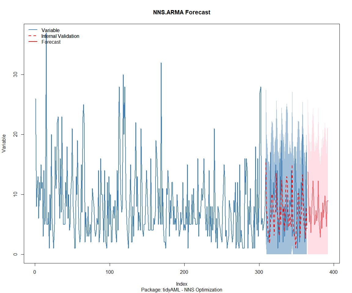
Package: tidyAML
[1] "CURRNET METHOD: lin"
[1] "COPY LATEST PARAMETERS DIRECTLY FOR NNS.ARMA() IF ERROR:"
[1] "NNS.ARMA(... method =  'lin' , seasonal.factor =  c( 5 ) ...)"
[1] "CURRENT lin OBJECTIVE FUNCTION = 19.9598264657801"
[1] "BEST method = 'lin' PATH MEMBER = c( 5 )"
[1] "BEST lin OBJECTIVE FUNCTION = 19.9598264657801"
[1] "CURRNET METHOD: nonlin"
[1] "COPY LATEST PARAMETERS DIRECTLY FOR NNS.ARMA() IF ERROR:"
[1] "NNS.ARMA(... method =  'nonlin' , seasonal.factor =  c( 5 ) ...)"
[1] "CURRENT nonlin OBJECTIVE FUNCTION = 16.0998631826203"
[1] "BEST method = 'nonlin' PATH MEMBER = c( 5 )"
[1] "BEST nonlin OBJECTIVE FUNCTION = 16.0998631826203"
[1] "CURRNET METHOD: both"
[1] "COPY LATEST PARAMETERS DIRECTLY FOR NNS.ARMA() IF ERROR:"
[1] "NNS.ARMA(... method =  'both' , seasonal.factor =  c( 5 ) ...)"
[1] "CURRENT both OBJECTIVE FUNCTION = 16.0461051437667"
[1] "BEST method = 'both' PATH MEMBER = c( 5 )"
[1] "BEST both OBJECTIVE FUNCTION = 16.0461051437667"
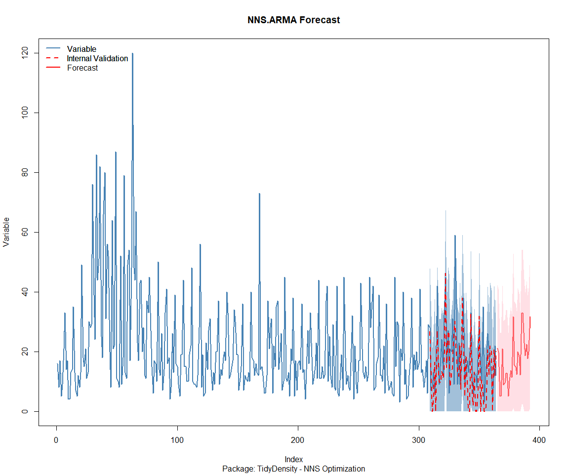
Package: TidyDensity
[1] "CURRNET METHOD: lin"
[1] "COPY LATEST PARAMETERS DIRECTLY FOR NNS.ARMA() IF ERROR:"
[1] "NNS.ARMA(... method =  'lin' , seasonal.factor =  c( 2 ) ...)"
[1] "CURRENT lin OBJECTIVE FUNCTION = 15.7588952235301"
[1] "BEST method = 'lin' PATH MEMBER = c( 2 )"
[1] "BEST lin OBJECTIVE FUNCTION = 15.7588952235301"
[1] "CURRNET METHOD: nonlin"
[1] "COPY LATEST PARAMETERS DIRECTLY FOR NNS.ARMA() IF ERROR:"
[1] "NNS.ARMA(... method =  'nonlin' , seasonal.factor =  c( 2 ) ...)"
[1] "CURRENT nonlin OBJECTIVE FUNCTION = 8.53359704187728"
[1] "BEST method = 'nonlin' PATH MEMBER = c( 2 )"
[1] "BEST nonlin OBJECTIVE FUNCTION = 8.53359704187728"
[1] "CURRNET METHOD: both"
[1] "COPY LATEST PARAMETERS DIRECTLY FOR NNS.ARMA() IF ERROR:"
[1] "NNS.ARMA(... method =  'both' , seasonal.factor =  c( 2 ) ...)"
[1] "CURRENT both OBJECTIVE FUNCTION = 11.0065491243488"
[1] "BEST method = 'both' PATH MEMBER = c( 2 )"
[1] "BEST both OBJECTIVE FUNCTION = 11.0065491243488"
[[1]]
NULL

[[2]]
NULL

[[3]]
NULL

[[4]]
NULL

[[5]]
NULL

[[6]]
NULL

[[7]]
NULL

[[8]]
NULL
Pre-Processing
Now we are going to do some basic pre-processing.
data_padded_tbl <- base_data %>%
  pad_by_time(
    .date_var  = date,
    .pad_value = 0
  )

# Get log interval and standardization parameters
log_params  <- liv(data_padded_tbl$value, limit_lower = 0, offset = 1, silent = TRUE)
limit_lower <- log_params$limit_lower
limit_upper <- log_params$limit_upper
offset      <- log_params$offset

data_liv_tbl <- data_padded_tbl %>%
  # Get log interval transform
  mutate(value_trans = liv(value, limit_lower = 0, offset = 1, silent = TRUE)$log_scaled)

# Get Standardization Params
std_params <- standard_vec(data_liv_tbl$value_trans, silent = TRUE)
std_mean   <- std_params$mean
std_sd     <- std_params$sd

data_transformed_tbl <- data_liv_tbl %>%
  group_by(package) %>%
  # get standardization
  mutate(value_trans = standard_vec(value_trans, silent = TRUE)$standard_scaled) %>%
  tk_augment_fourier(
    .date_var = date,
    .periods  = c(7, 14, 30, 90, 180),
    .K        = 2
  ) %>%
  tk_augment_timeseries_signature(
    .date_var = date
  ) %>%
  ungroup() %>%
  select(-c(value, -year.iso))
Since this is panel data we can follow one of two different modeling strategies. We can search for a global model in the panel data or we can use nested forecasting finding the best model for each of the time series. Since we only have 5 panels, we will use nested forecasting.
To do this we will use the nest_timeseries and
split_nested_timeseries functions to create a nested tibble.
horizon <- 4*7

nested_data_tbl <- data_transformed_tbl %>%

    # 0. Filter out column where package is NA
    filter(!is.na(package)) %>%

    # 1. Extending: We'll predict n days into the future.
    extend_timeseries(
        .id_var        = package,
        .date_var      = date,
        .length_future = horizon
    ) %>%

    # 2. Nesting: We'll group by id, and create a future dataset
    #    that forecasts n days of extended data and
    #    an actual dataset that contains n*2 days
    nest_timeseries(
        .id_var        = package,
        .length_future = horizon
        #.length_actual = horizon*2
    ) %>%

   # 3. Splitting: We'll take the actual data and create splits
   #    for accuracy and confidence interval estimation of n das (test)
   #    and the rest is training data
    split_nested_timeseries(
        .length_test = horizon
    )

nested_data_tbl
# A tibble: 8 × 4
  package       .actual_data          .future_data       .splits
  <fct>         <list>                <list>             <list>
1 healthyR.data <tibble [2,028 × 50]> <tibble [28 × 50]> <split [2000|28]>
2 healthyR      <tibble [2,022 × 50]> <tibble [28 × 50]> <split [1994|28]>
3 healthyR.ts   <tibble [1,958 × 50]> <tibble [28 × 50]> <split [1930|28]>
4 healthyverse  <tibble [1,867 × 50]> <tibble [28 × 50]> <split [1839|28]>
5 healthyR.ai   <tibble [1,763 × 50]> <tibble [28 × 50]> <split [1735|28]>
6 TidyDensity   <tibble [1,616 × 50]> <tibble [28 × 50]> <split [1588|28]>
7 tidyAML       <tibble [1,220 × 50]> <tibble [28 × 50]> <split [1192|28]>
8 RandomWalker  <tibble [644 × 50]>   <tibble [28 × 50]> <split [616|28]>
Now it is time to make some recipes and models using the modeltime workflow.
Modeltime Workflow
Recipe Object
recipe_base <- recipe(
  value_trans ~ .
  , data = extract_nested_test_split(nested_data_tbl)
  )

recipe_base

recipe_date <- recipe(
  value_trans ~ date
  , data = extract_nested_test_split(nested_data_tbl)
  )
Models
# Models ------------------------------------------------------------------

# Auto ARIMA --------------------------------------------------------------

model_spec_arima_no_boost <- arima_reg() %>%
  set_engine(engine = "auto_arima")

wflw_auto_arima <- workflow() %>%
  add_recipe(recipe = recipe_date) %>%
  add_model(model_spec_arima_no_boost)

# NNETAR ------------------------------------------------------------------

model_spec_nnetar <- nnetar_reg(
  mode              = "regression"
  , seasonal_period = "auto"
) %>%
  set_engine("nnetar")

wflw_nnetar <- workflow() %>%
  add_recipe(recipe = recipe_base) %>%
  add_model(model_spec_nnetar)

# TSLM --------------------------------------------------------------------

model_spec_lm <- linear_reg() %>%
  set_engine("lm")

wflw_lm <- workflow() %>%
  add_recipe(recipe = recipe_base) %>%
  add_model(model_spec_lm)

# MARS --------------------------------------------------------------------

model_spec_mars <- mars(mode = "regression") %>%
  set_engine("earth")

wflw_mars <- workflow() %>%
  add_recipe(recipe = recipe_date) %>%
  add_model(model_spec_mars)
Nested Modeltime Tables
nested_modeltime_tbl <- modeltime_nested_fit(
  # Nested Data
  nested_data = nested_data_tbl,
   control = control_nested_fit(
     verbose = TRUE,
     allow_par = FALSE
   ),
  # Add workflows
  wflw_auto_arima,
  wflw_lm,
  wflw_mars,
  wflw_nnetar
)
nested_modeltime_tbl <- nested_modeltime_tbl[!is.na(nested_modeltime_tbl$package),]
Model Accuracy
nested_modeltime_tbl %>%
  extract_nested_test_accuracy() %>%
  filter(!is.na(package)) %>%
  knitr::kable()
| package | .model_id | .model_desc | .type | mae | mape | mase | smape | rmse | rsq |
|---|---|---|---|---|---|---|---|---|---|
| healthyR.data | 1 | ARIMA | Test | 0.7507465 | 149.54051 | 0.8303418 | 168.32934 | 0.9007544 | 0.0484576 |
| healthyR.data | 2 | LM | Test | 0.8732312 | 194.63564 | 0.9658125 | 162.98138 | 1.0330344 | 0.0120811 |
| healthyR.data | 3 | EARTH | Test | 0.7575491 | 130.59834 | 0.8378657 | 171.52345 | 0.9141952 | 0.0302500 |
| healthyR.data | 4 | NNAR | Test | 0.8759601 | 230.27420 | 0.9688308 | 164.67328 | 1.0217325 | 0.0000100 |
| healthyR | 1 | ARIMA | Test | 0.8488584 | 153.13237 | 0.8265312 | 144.68537 | 1.0729126 | 0.0246230 |
| healthyR | 2 | LM | Test | 0.9083792 | 474.68581 | 0.8844865 | 156.28409 | 1.0771707 | 0.0060977 |
| healthyR | 3 | EARTH | Test | 0.8924920 | 483.99757 | 0.8690171 | 144.37554 | 1.0901875 | 0.0754972 |
| healthyR | 4 | NNAR | Test | 0.7949938 | 500.98993 | 0.7740835 | 145.89320 | 0.9747028 | 0.0638250 |
| healthyR.ts | 1 | ARIMA | Test | 0.7361228 | 541.22287 | 0.6842751 | 184.22678 | 0.9737209 | 0.0626182 |
| healthyR.ts | 2 | LM | Test | 0.8067217 | 8045.09227 | 0.7499015 | 152.45402 | 1.0420178 | 0.0174505 |
| healthyR.ts | 3 | EARTH | Test | 0.8035446 | 8491.30948 | 0.7469482 | 133.87636 | 1.0389016 | 0.0587625 |
| healthyR.ts | 4 | NNAR | Test | 0.8103483 | 8638.99681 | 0.7532727 | 158.88129 | 1.0155394 | 0.0002010 |
| healthyverse | 1 | ARIMA | Test | 0.5975302 | 80.69445 | 0.8106795 | 48.96968 | 0.6949792 | 0.0093003 |
| healthyverse | 2 | LM | Test | 0.7800006 | 57.42363 | 1.0582403 | 70.19892 | 0.9347424 | 0.0479186 |
| healthyverse | 3 | EARTH | Test | 0.5474307 | 92.44469 | 0.7427087 | 43.52108 | 0.7041679 | 0.0117119 |
| healthyverse | 4 | NNAR | Test | 0.8462870 | 61.97447 | 1.1481722 | 81.48836 | 1.0095693 | 0.0368411 |
| healthyR.ai | 1 | ARIMA | Test | 0.8365606 | 135.88214 | 0.9564851 | 131.46884 | 1.0265235 | 0.0385271 |
| healthyR.ai | 2 | LM | Test | 0.8455540 | 161.83936 | 0.9667678 | 118.53349 | 1.0468575 | 0.0276788 |
| healthyR.ai | 3 | EARTH | Test | 1.2235298 | 236.17876 | 1.3989281 | 124.91379 | 1.4880907 | 0.1364629 |
| healthyR.ai | 4 | NNAR | Test | 0.8261302 | 130.66741 | 0.9445596 | 139.33391 | 0.9849934 | 0.0103299 |
| TidyDensity | 1 | ARIMA | Test | 0.8763617 | 297.91511 | 0.6926909 | 156.91743 | 1.0198544 | 0.0000623 |
| TidyDensity | 2 | LM | Test | 0.8708826 | 391.63429 | 0.6883601 | 148.20724 | 1.0380858 | 0.0027765 |
| TidyDensity | 3 | EARTH | Test | 0.8105451 | 137.64568 | 0.6406683 | 165.84572 | 1.0077440 | 0.1857907 |
| TidyDensity | 4 | NNAR | Test | 0.8977241 | 398.51221 | 0.7095760 | 147.87805 | 1.0808204 | 0.0000742 |
| tidyAML | 1 | ARIMA | Test | 0.9437645 | 99.52105 | 0.8409744 | 147.18870 | 1.1672789 | 0.0462231 |
| tidyAML | 2 | LM | Test | 1.1898474 | 237.05891 | 1.0602551 | 132.14142 | 1.4406685 | 0.0631144 |
| tidyAML | 3 | EARTH | Test | 0.9346513 | 107.58686 | 0.8328537 | 166.79732 | 1.1209699 | 0.0536250 |
| tidyAML | 4 | NNAR | Test | 0.9650151 | 140.62069 | 0.8599104 | 148.01156 | 1.1815581 | 0.0238534 |
| RandomWalker | 1 | ARIMA | Test | 0.8402987 | 115.97469 | 0.6905052 | 150.45194 | 1.0149964 | 0.0268493 |
| RandomWalker | 2 | LM | Test | 0.8467263 | 152.59793 | 0.6957870 | 158.37744 | 1.0410025 | 0.0009438 |
| RandomWalker | 3 | EARTH | Test | 0.8418871 | 95.83054 | 0.6918104 | 181.87265 | 1.0164836 | 0.0219543 |
| RandomWalker | 4 | NNAR | Test | 1.0027013 | 139.17405 | 0.8239574 | 157.05108 | 1.2141923 | 0.1017852 |
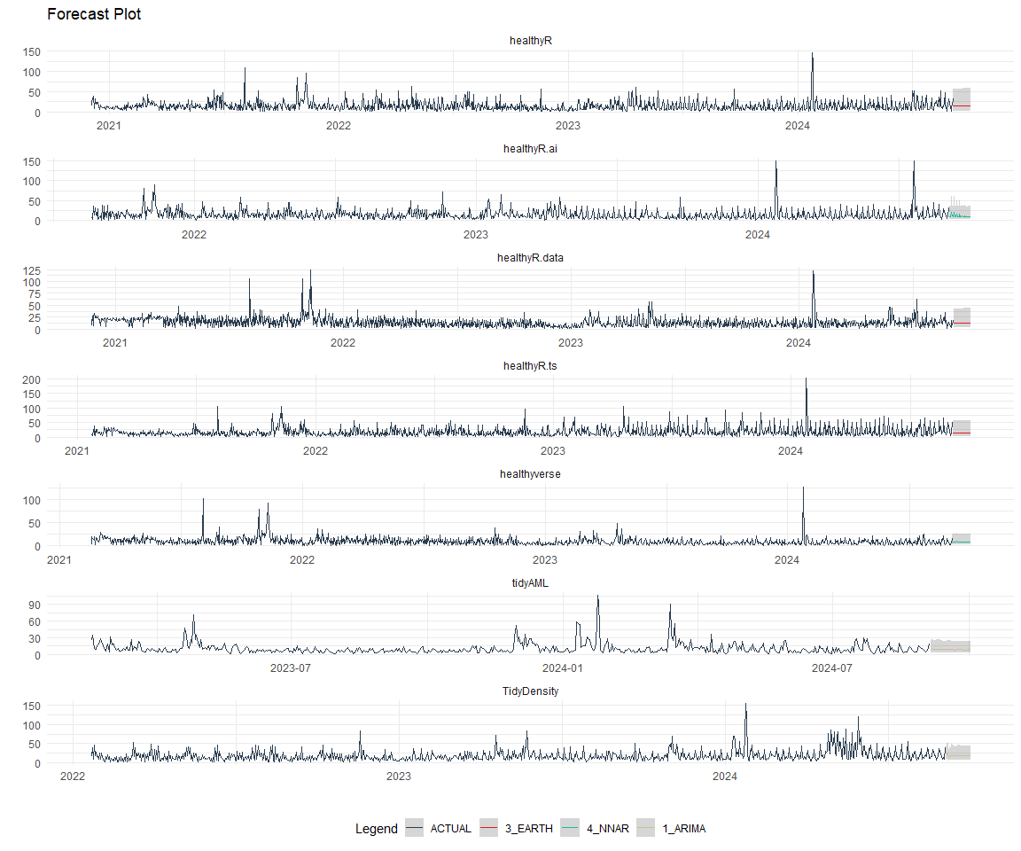
Plot Models
nested_modeltime_tbl %>%
  extract_nested_test_forecast() %>%
  group_by(package) %>%
  filter_by_time(.date_var = .index, .start_date = max(.index) - 60) %>%
  ungroup() %>%
  plot_modeltime_forecast(
    .interactive = FALSE,
    .conf_interval_show  = FALSE,
    .facet_scales = "free"
  ) +
  theme_minimal() +
  facet_wrap(~ package, nrow = 3) +
  theme(legend.position = "bottom")

Best Model
best_nested_modeltime_tbl <- nested_modeltime_tbl %>%
  modeltime_nested_select_best(
    metric = "rmse",
    minimize = TRUE,
    filter_test_forecasts = TRUE
  )

best_nested_modeltime_tbl %>%
  extract_nested_best_model_report()
# Nested Modeltime Table


# A tibble: 8 × 10
  package      .model_id .model_desc .type   mae  mape  mase smape  rmse     rsq
  <fct>            <int> <chr>       <chr> <dbl> <dbl> <dbl> <dbl> <dbl>   <dbl>
1 healthyR.da…         1 ARIMA       Test  0.751 150.  0.830 168.  0.901 0.0485
2 healthyR             4 NNAR        Test  0.795 501.  0.774 146.  0.975 0.0638
3 healthyR.ts          1 ARIMA       Test  0.736 541.  0.684 184.  0.974 0.0626
4 healthyverse         1 ARIMA       Test  0.598  80.7 0.811  49.0 0.695 0.00930
5 healthyR.ai          4 NNAR        Test  0.826 131.  0.945 139.  0.985 0.0103
6 TidyDensity          3 EARTH       Test  0.811 138.  0.641 166.  1.01  0.186
7 tidyAML              3 EARTH       Test  0.935 108.  0.833 167.  1.12  0.0536
8 RandomWalker         1 ARIMA       Test  0.840 116.  0.691 150.  1.01  0.0268
best_nested_modeltime_tbl %>%
  extract_nested_test_forecast() %>%
  #filter(!is.na(.model_id)) %>%
  group_by(package) %>%
  filter_by_time(.date_var = .index, .start_date = max(.index) - 60) %>%
  ungroup() %>%
  plot_modeltime_forecast(
    .interactive = FALSE,
    .conf_interval_alpha = 0.2,
    .facet_scales = "free"
  ) +
  facet_wrap(~ package, nrow = 3) +
  theme_minimal() +
  theme(legend.position = "bottom")
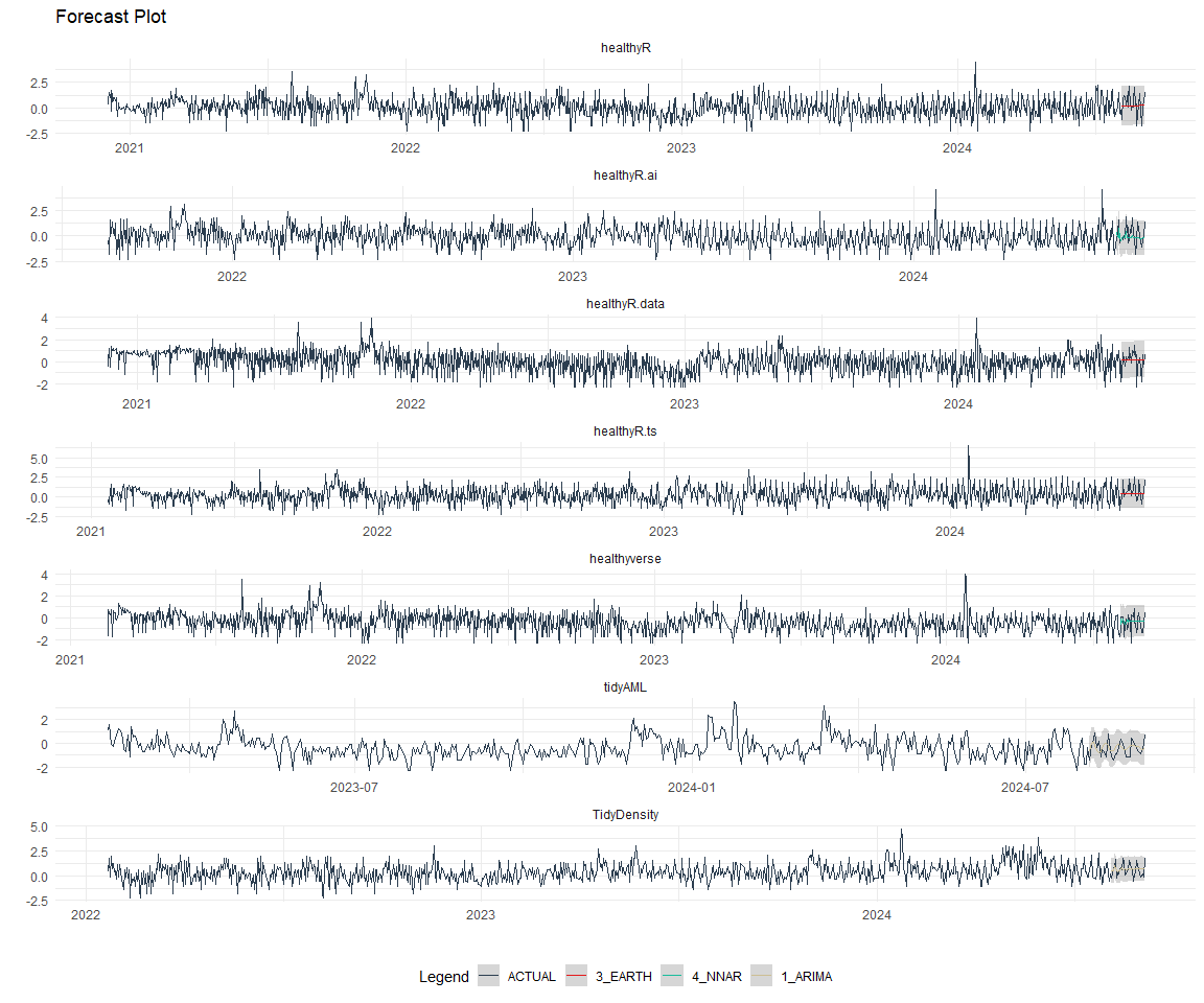
Refitting and Future Forecast
Now that we have the best models, we can make our future forecasts.
nested_modeltime_refit_tbl <- best_nested_modeltime_tbl %>%
    modeltime_nested_refit(
        control = control_nested_refit(verbose = TRUE)
    )
nested_modeltime_refit_tbl
# Nested Modeltime Table


# A tibble: 8 × 5
  package       .actual_data .future_data .splits           .modeltime_tables
  <fct>         <list>       <list>       <list>            <list>
1 healthyR.data <tibble>     <tibble>     <split [2000|28]> <mdl_tm_t [1 × 5]>
2 healthyR      <tibble>     <tibble>     <split [1994|28]> <mdl_tm_t [1 × 5]>
3 healthyR.ts   <tibble>     <tibble>     <split [1930|28]> <mdl_tm_t [1 × 5]>
4 healthyverse  <tibble>     <tibble>     <split [1839|28]> <mdl_tm_t [1 × 5]>
5 healthyR.ai   <tibble>     <tibble>     <split [1735|28]> <mdl_tm_t [1 × 5]>
6 TidyDensity   <tibble>     <tibble>     <split [1588|28]> <mdl_tm_t [1 × 5]>
7 tidyAML       <tibble>     <tibble>     <split [1192|28]> <mdl_tm_t [1 × 5]>
8 RandomWalker  <tibble>     <tibble>     <split [616|28]>  <mdl_tm_t [1 × 5]>
nested_modeltime_refit_tbl %>%
  extract_nested_future_forecast() %>%
  group_by(package) %>%
  mutate(across(.value:.conf_hi, .fns = ~ standard_inv_vec(
    x    = .,
    mean = std_mean,
    sd   = std_sd
  )$standard_inverse_value)) %>%
  mutate(across(.value:.conf_hi, .fns = ~ liiv(
    x = .,
    limit_lower = limit_lower,
    limit_upper = limit_upper,
    offset      = offset
  )$rescaled_v)) %>%
  filter_by_time(.date_var = .index, .start_date = max(.index) - 60) %>%
  ungroup() %>%
  plot_modeltime_forecast(
    .interactive = FALSE,
    .conf_interval_alpha = 0.2,
    .facet_scales = "free"
  ) +
  facet_wrap(~ package, nrow = 3) +
  theme_minimal() +
  theme(legend.position = "bottom")