package-downloads
CRAN Downloads
Steven P. Sanderson II, MPH - Date: 18 April, 2025
This repo contains the analysis of downloads of my R packages:
All of which follow the “analyses as
package”
philosophy this repo itself is an R package that can installed using
remotes::install_github().
I have forked this project itself from
ggcharts-analysis.
While I analyze healthyverse packages here, the functions are written
in a way that you can analyze any CRAN package with a slight
modification to the download_log function.
This file was last updated on April 18, 2025.
library(packagedownloads)
library(tidyverse)
library(patchwork)
library(timetk)
library(knitr)
library(leaflet)
library(htmltools)
library(tmaptools)
library(mapview)
library(countrycode)
library(htmlwidgets)
library(webshot)
library(rmarkdown)
library(dtplyr)
start_date      <- Sys.Date() - 9 #as.Date("2020-11-15")
end_date        <- Sys.Date() - 2
total_downloads <- download_logs(start_date, end_date)
interactive     <- FALSE
pkg_release_date_tbl()
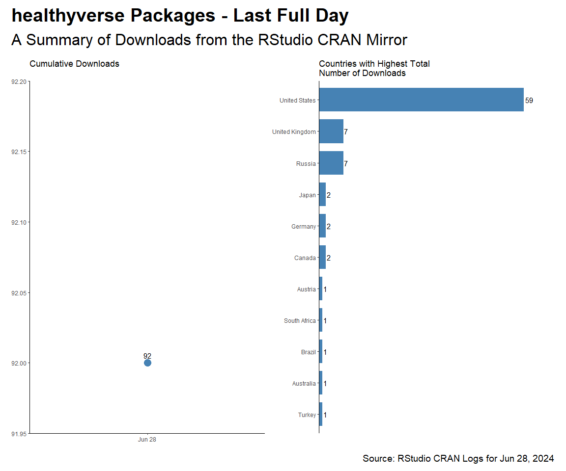
Last Full Day Data
downloads            <- total_downloads |> filter(date == max(date))
daily_downloads      <- compute_daily_downloads(downloads)
downloads_by_country <- compute_downloads_by_country(downloads)

p1 <- plot_cumulative_downloads(daily_downloads)
p2 <- plot_downloads_by_country(downloads_by_country)

f <- function(date) format(date, "%b %d, %Y")
patchwork_theme <- theme_classic(base_size = 24) +
  theme(
    plot.title   = element_text(face = "bold"),
    plot.caption = element_text(size = 14)
  )
p1 + p2 +
  plot_annotation(
    title    = "healthyverse Packages - Last Full Day",
    subtitle = "A Summary of Downloads from the RStudio CRAN Mirror",
    caption  = glue::glue("Source: RStudio CRAN Logs for {f(end_date)}"),
    theme    = patchwork_theme
  )
downloads |>
  count(package, version) |>
  tidyr::pivot_wider(
    id_cols       = version
    , names_from  = package
    , values_from = n
    , values_fill = 0
    ) |>
  arrange(version) |>
  kable()
| version | RandomWalker | TidyDensity | healthyR | healthyR.ai | healthyR.data | healthyR.ts | healthyverse | tidyAML |
|---|---|---|---|---|---|---|---|---|
| 0.0.1 | 0 | 0 | 0 | 1 | 0 | 0 | 0 | 0 |
| 0.0.11 | 0 | 0 | 0 | 2 | 0 | 0 | 0 | 0 |
| 0.0.12 | 0 | 0 | 0 | 1 | 0 | 0 | 0 | 0 |
| 0.0.2 | 0 | 0 | 0 | 1 | 0 | 0 | 0 | 1 |
| 0.0.3 | 0 | 0 | 0 | 1 | 0 | 0 | 0 | 0 |
| 0.0.4 | 0 | 0 | 0 | 0 | 0 | 0 | 0 | 1 |
| 0.0.5 | 0 | 0 | 0 | 0 | 0 | 0 | 0 | 13 |
| 0.0.6 | 0 | 0 | 0 | 1 | 0 | 0 | 0 | 0 |
| 0.0.7 | 0 | 0 | 0 | 1 | 0 | 0 | 0 | 0 |
| 0.0.8 | 0 | 0 | 0 | 1 | 0 | 0 | 0 | 0 |
| 0.1.0 | 0 | 0 | 0 | 13 | 0 | 0 | 0 | 0 |
| 0.1.1 | 0 | 0 | 0 | 0 | 0 | 1 | 0 | 0 |
| 0.1.4 | 0 | 0 | 0 | 0 | 0 | 1 | 0 | 0 |
| 0.1.6 | 0 | 0 | 0 | 0 | 0 | 1 | 0 | 0 |
| 0.1.7 | 0 | 0 | 0 | 0 | 0 | 1 | 0 | 0 |
| 0.1.9 | 0 | 0 | 0 | 0 | 0 | 1 | 0 | 0 |
| 0.2.0 | 11 | 0 | 0 | 0 | 0 | 0 | 0 | 0 |
| 0.2.10 | 0 | 0 | 0 | 0 | 0 | 1 | 0 | 0 |
| 0.2.2 | 0 | 0 | 15 | 0 | 0 | 1 | 0 | 0 |
| 0.2.3 | 0 | 0 | 0 | 0 | 0 | 1 | 0 | 0 |
| 0.2.4 | 0 | 0 | 0 | 0 | 0 | 1 | 0 | 0 |
| 0.2.5 | 0 | 0 | 0 | 0 | 0 | 1 | 0 | 0 |
| 0.2.6 | 0 | 0 | 0 | 0 | 0 | 1 | 0 | 0 |
| 0.2.7 | 0 | 0 | 0 | 0 | 0 | 1 | 0 | 0 |
| 0.2.8 | 0 | 0 | 0 | 0 | 0 | 1 | 0 | 0 |
| 0.2.9 | 0 | 0 | 0 | 0 | 0 | 1 | 0 | 0 |
| 0.3.1 | 0 | 0 | 0 | 0 | 0 | 12 | 0 | 0 |
| 1.0.0 | 0 | 0 | 0 | 0 | 1 | 0 | 0 | 0 |
| 1.0.1 | 0 | 0 | 0 | 0 | 1 | 0 | 0 | 0 |
| 1.0.2 | 0 | 0 | 0 | 0 | 1 | 0 | 0 | 0 |
| 1.0.3 | 0 | 0 | 0 | 0 | 1 | 0 | 0 | 0 |
| 1.1.0 | 0 | 0 | 0 | 0 | 1 | 0 | 10 | 0 |
| 1.1.1 | 0 | 0 | 0 | 0 | 1 | 0 | 0 | 0 |
| 1.2.0 | 0 | 0 | 0 | 0 | 12 | 0 | 0 | 0 |
| 1.5.0 | 0 | 23 | 0 | 0 | 0 | 0 | 0 | 0 |
downloads |>
  count(package, sort = TRUE) |>
  tidyr::pivot_wider(
    names_from = package,
    values_from = n,
    values_fill = 0
  ) |>
  kable()
| healthyR.ts | TidyDensity | healthyR.ai | healthyR.data | healthyR | tidyAML | RandomWalker | healthyverse |
|---|---|---|---|---|---|---|---|
| 26 | 23 | 22 | 18 | 15 | 15 | 11 | 10 |
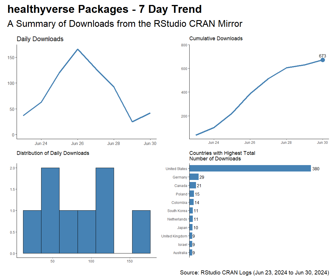
Current Trend
Here are the current 7 day trends for the healthyverse suite of
packages.
downloads            <- total_downloads[date >= start_date]
daily_downloads      <- compute_daily_downloads(downloads)
downloads_by_country <- compute_downloads_by_country(downloads)

p1 <- plot_daily_downloads(daily_downloads)
p2 <- plot_cumulative_downloads(daily_downloads)
p3 <- hist_daily_downloads(daily_downloads)
p4 <- plot_downloads_by_country(downloads_by_country)

f <- function(date) format(date, "%b %d, %Y")
patchwork_theme <- theme_classic(base_size = 24) +
  theme(
    plot.title   = element_text(face = "bold"),
    plot.caption = element_text(size = 14)
  )
p1 + p2 + p3 + p4 +
  plot_annotation(
    title    = "healthyverse Packages - 7 Day Trend",
    subtitle = "A Summary of Downloads from the RStudio CRAN Mirror",
    caption  = glue::glue("Source: RStudio CRAN Logs ({f(start_date)} to {f(end_date)})"),
    theme    = patchwork_theme
  )
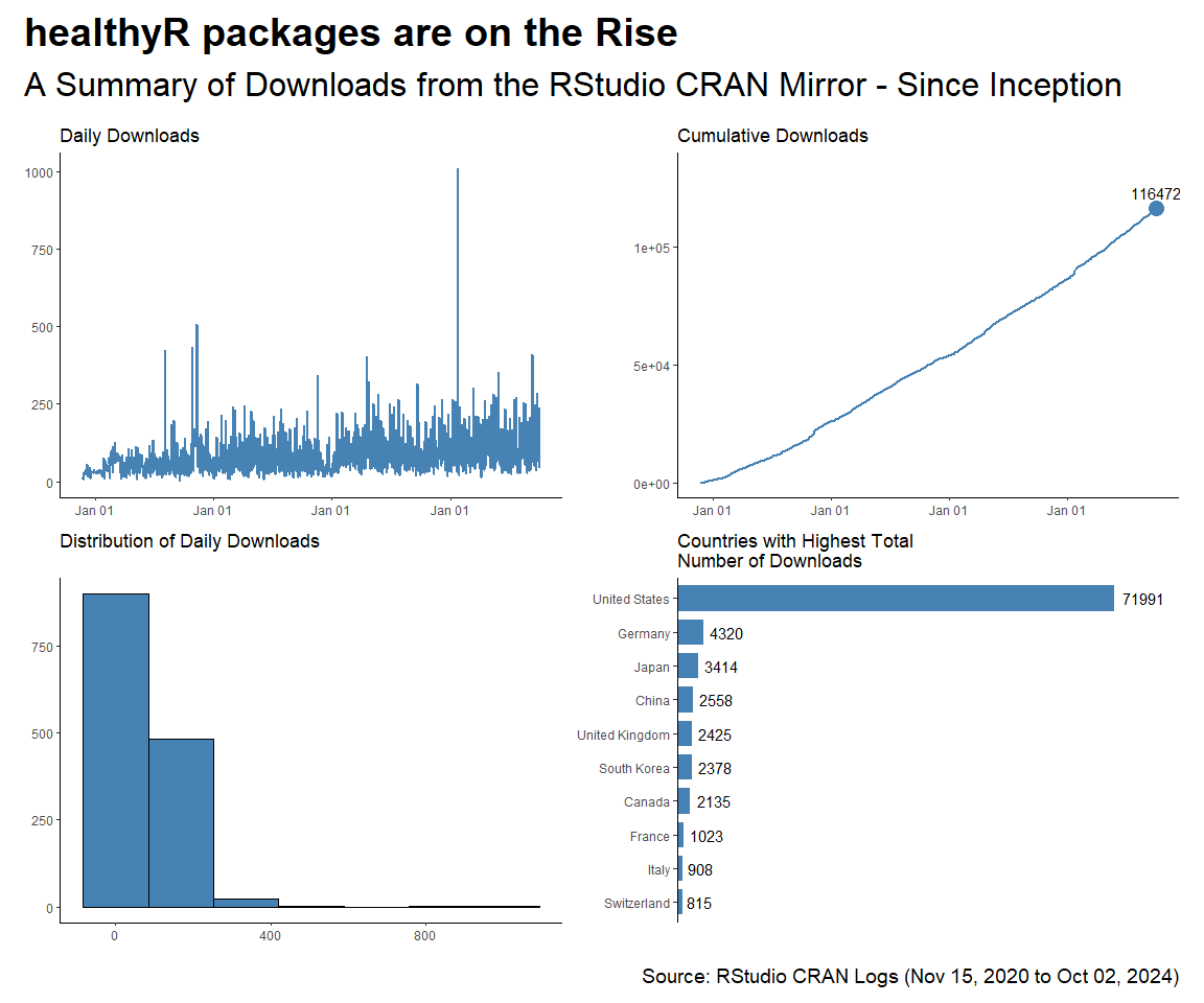
Since Inception
start_date <- as.Date("2020-11-15")

daily_downloads <- compute_daily_downloads(downloads = total_downloads)
downloads_by_country <- compute_downloads_by_country(downloads = total_downloads)

p1 <- plot_daily_downloads(daily_downloads)
p2 <- plot_cumulative_downloads(daily_downloads)
p3 <- hist_daily_downloads(daily_downloads)
p4 <- plot_downloads_by_country(downloads_by_country)

f <- function(date) format(date, "%b %d, %Y")
patchwork_theme <- theme_classic(base_size = 24) +
  theme(
    plot.title   = element_text(face = "bold"),
    plot.caption = element_text(size = 14)
  )
p1 + p2 + p3 + p4 +
  plot_annotation(
    title    = "healthyR packages are on the Rise",
    subtitle = "A Summary of Downloads from the RStudio CRAN Mirror - Since Inception",
    caption  = glue::glue("Source: RStudio CRAN Logs ({f(start_date)} to {f(end_date)})"),
    theme    = patchwork_theme
  )
By Release Date
pkg_tbl <- readRDS("pkg_release_tbl.rds")
dl_tbl <- total_downloads %>%
    filter(
    date != "2024-05-29" &
      !(date == "2024-06-12" & package == "TidyDensity")
    ) |> # bad data on this for some reason
  group_by(package) %>%
  summarise_by_time(
    .date_var = date,
    .by = "week",
    N = n()
  ) %>%
  ungroup() %>%
  select(date, package, N)

dl_tbl %>%
ggplot(aes(date, log1p(N))) +
  theme_bw() +
  geom_point(aes(group = package, color = package), size = 1) +
  geom_line(aes(group = package, color = package)) +
  ggtitle(paste("Package Downloads: {healthyverse}")) +
  geom_smooth(method = "loess", color = "black",  se = FALSE) +
  geom_vline(
    data = pkg_tbl
    , aes(xintercept = as.numeric(date))
    , color = "red"
    , lwd = 1
    , lty = "solid"
  ) +
  facet_wrap(package ~., ncol = 2, scales = "free_x") +
  theme_minimal() +
  labs(
    subtitle = "Vertical lines represent release dates",
    x = "Date",
    y = "log1p(Counts)",
    color = "Package"
  ) +
  theme(legend.position = "bottom")

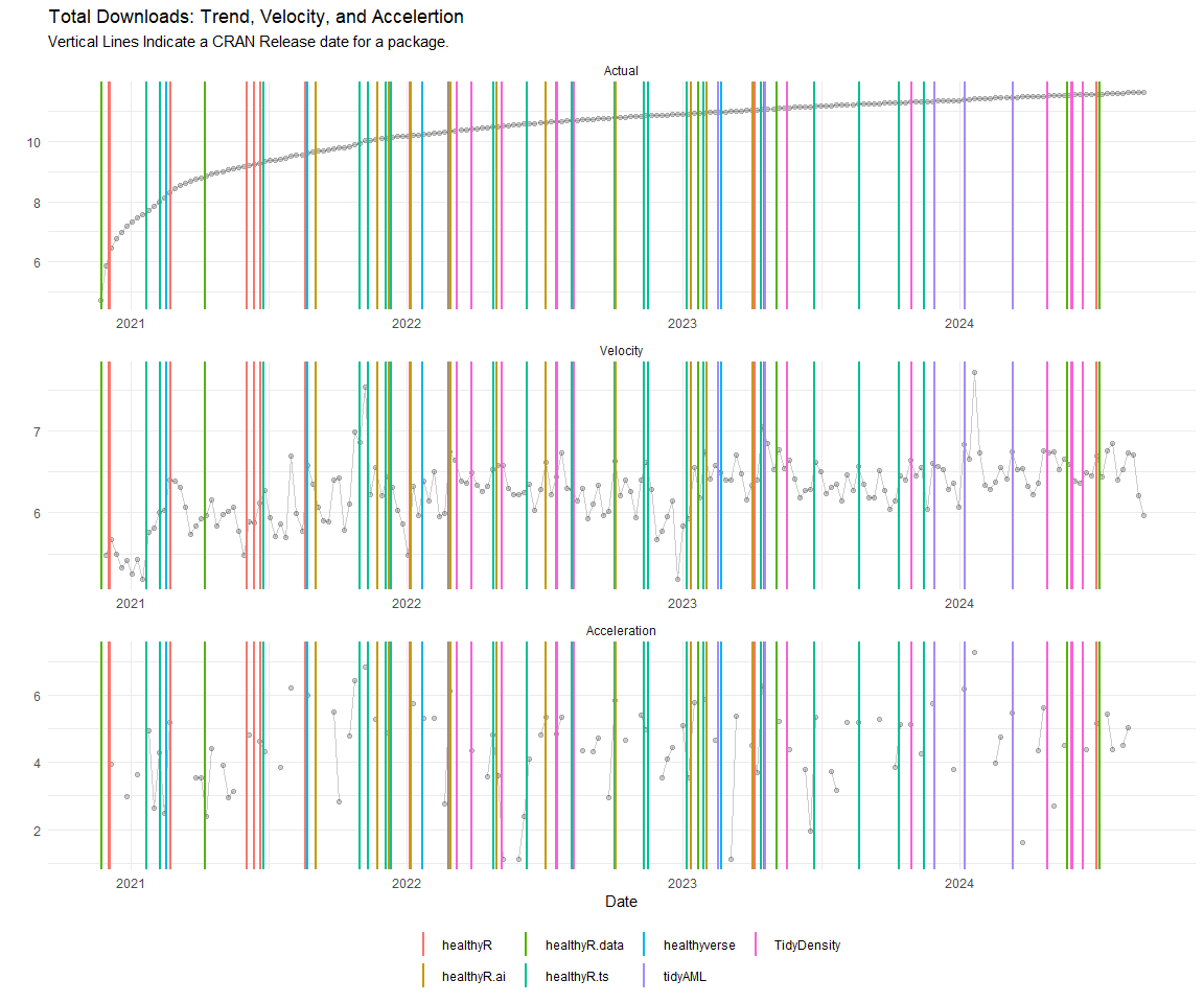
dl_tbl %>%
  select(date, N) %>%
  summarise_by_time(
    .date_var = date,
    .by = "week",
    Actual = sum(N, na.rm = TRUE)
  ) %>%
  mutate(Actual = cumsum(Actual)) %>%
  tk_augment_differences(.value = Actual, .differences = 1) %>%
  tk_augment_differences(.value = Actual, .differences = 2) %>%
  rename(velocity = contains("_diff1")) %>%
  rename(acceleration = contains("_diff2")) %>%
  pivot_longer(-date) %>%
  mutate(name = str_to_title(name)) %>%
  mutate(name = as_factor(name)) %>%
  ggplot(aes(x = date, y = log1p(value), group = name)) +
  geom_point(alpha = .2) +
  geom_line(alpha = .2) +
  geom_vline(
    data = pkg_tbl
    , aes(xintercept = as.numeric(date), color = package)
    , lwd = 1
    , lty = "solid"
  ) +
  facet_wrap(name ~ ., ncol = 1, scale = "free") +
  theme_minimal() +
  labs(
    title = "Total Downloads: Trend, Velocity, and Accelertion",
    subtitle = "Vertical Lines Indicate a CRAN Release date for a package.",
    x = "Date",
    y = "",
    color = ""
  ) +
  theme(legend.position = "bottom")
Map of Downloads
A leaflet map of countries where a package has been downloaded.
mapping_dataset() %>%
  head() %>%
  knitr::kable()
| country | latitude | longitude | display_name | icon |
|---|---|---|---|---|
| United States | 39.78373 | -100.445882 | United States | https://nominatim.openstreetmap.org/ui/mapicons/poi_boundary_administrative.p.20.png |
| United Kingdom | 54.70235 | -3.276575 | United Kingdom | https://nominatim.openstreetmap.org/ui/mapicons/poi_boundary_administrative.p.20.png |
| Germany | 51.16382 | 10.447831 | Deutschland | https://nominatim.openstreetmap.org/ui/mapicons/poi_boundary_administrative.p.20.png |
| Hong Kong SAR China | 22.35063 | 114.184916 | 香港 Hong Kong, 中国 | https://nominatim.openstreetmap.org/ui/mapicons/poi_boundary_administrative.p.20.png |
| Japan | 36.57484 | 139.239418 | 日本 | https://nominatim.openstreetmap.org/ui/mapicons/poi_boundary_administrative.p.20.png |
| Chile | -31.76134 | -71.318770 | Chile | https://nominatim.openstreetmap.org/ui/mapicons/poi_boundary_administrative.p.20.png |
l <- map_leaflet()
saveWidget(l, "downloads_map.html")
webshot("downloads_map.html", file = "map.png",
        cliprect = "viewport")
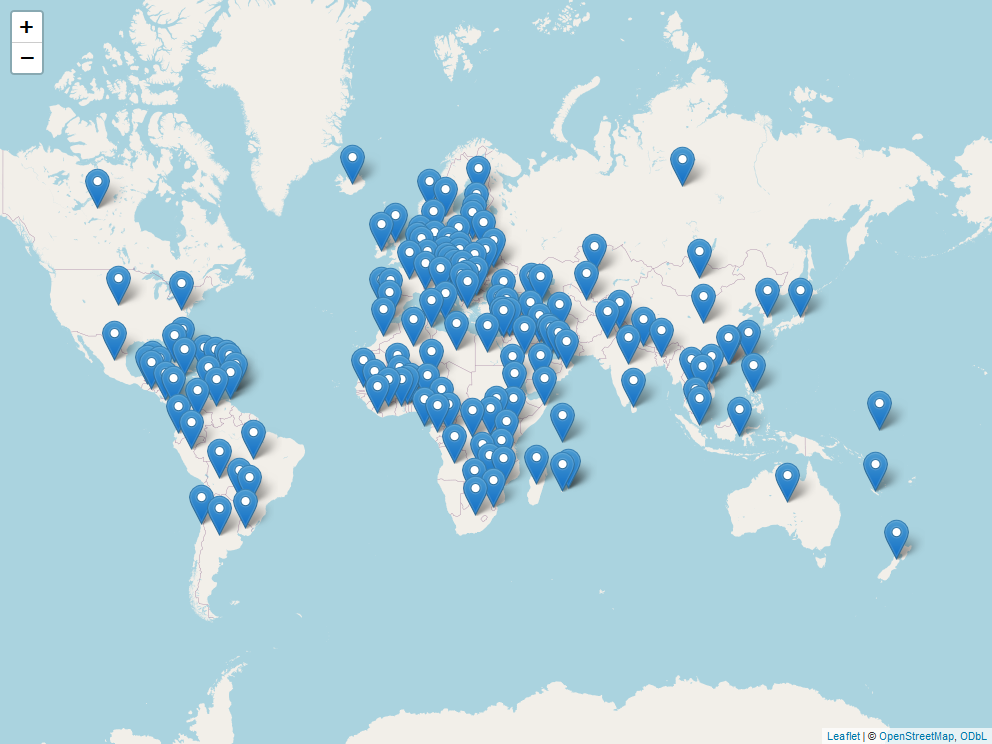
To date there has been downloads in a total of 159 different countries.
Analysis by Package
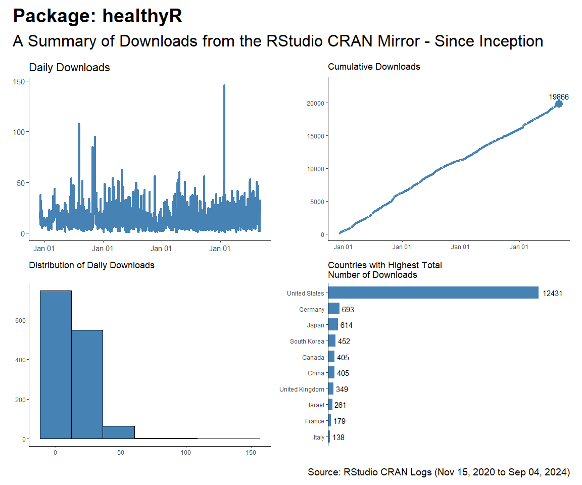
healthyR
start_date <- as.Date("2020-11-15")
pkg <- "healthyR"

daily_downloads <- compute_daily_downloads(
  downloads = total_downloads
  , pkg = pkg)
downloads_by_country <- compute_downloads_by_country(
  downloads = total_downloads
  , pkg = pkg)

p1 <- plot_daily_downloads(daily_downloads)
p2 <- plot_cumulative_downloads(daily_downloads)
p3 <- hist_daily_downloads(daily_downloads)
p4 <- plot_downloads_by_country(downloads_by_country)

f <- function(date) format(date, "%b %d, %Y")
patchwork_theme <- theme_classic(base_size = 24) +
  theme(
    plot.title   = element_text(face = "bold"),
    plot.caption = element_text(size = 14)
  )
p1 + p2 + p3 + p4 +
  plot_annotation(
    title    = glue::glue("Package: {pkg}"),
    subtitle = "A Summary of Downloads from the RStudio CRAN Mirror - Since Inception",
    caption  = glue::glue("Source: RStudio CRAN Logs ({f(start_date)} to {f(end_date)})"),
    theme    = patchwork_theme
  )
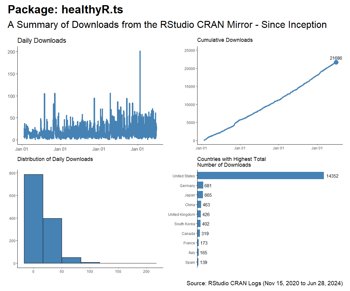
healthyR.ts
start_date <- as.Date("2020-11-15")
pkg <- "healthyR.ts"

daily_downloads <- compute_daily_downloads(
  downloads = total_downloads
  , pkg = pkg)
downloads_by_country <- compute_downloads_by_country(
  downloads = total_downloads
  , pkg = pkg)

p1 <- plot_daily_downloads(daily_downloads)
p2 <- plot_cumulative_downloads(daily_downloads)
p3 <- hist_daily_downloads(daily_downloads)
p4 <- plot_downloads_by_country(downloads_by_country)

f <- function(date) format(date, "%b %d, %Y")
patchwork_theme <- theme_classic(base_size = 24) +
  theme(
    plot.title   = element_text(face = "bold"),
    plot.caption = element_text(size = 14)
  )
p1 + p2 + p3 + p4 +
  plot_annotation(
    title    = glue::glue("Package: {pkg}"),
    subtitle = "A Summary of Downloads from the RStudio CRAN Mirror - Since Inception",
    caption  = glue::glue("Source: RStudio CRAN Logs ({f(start_date)} to {f(end_date)})"),
    theme    = patchwork_theme
  )
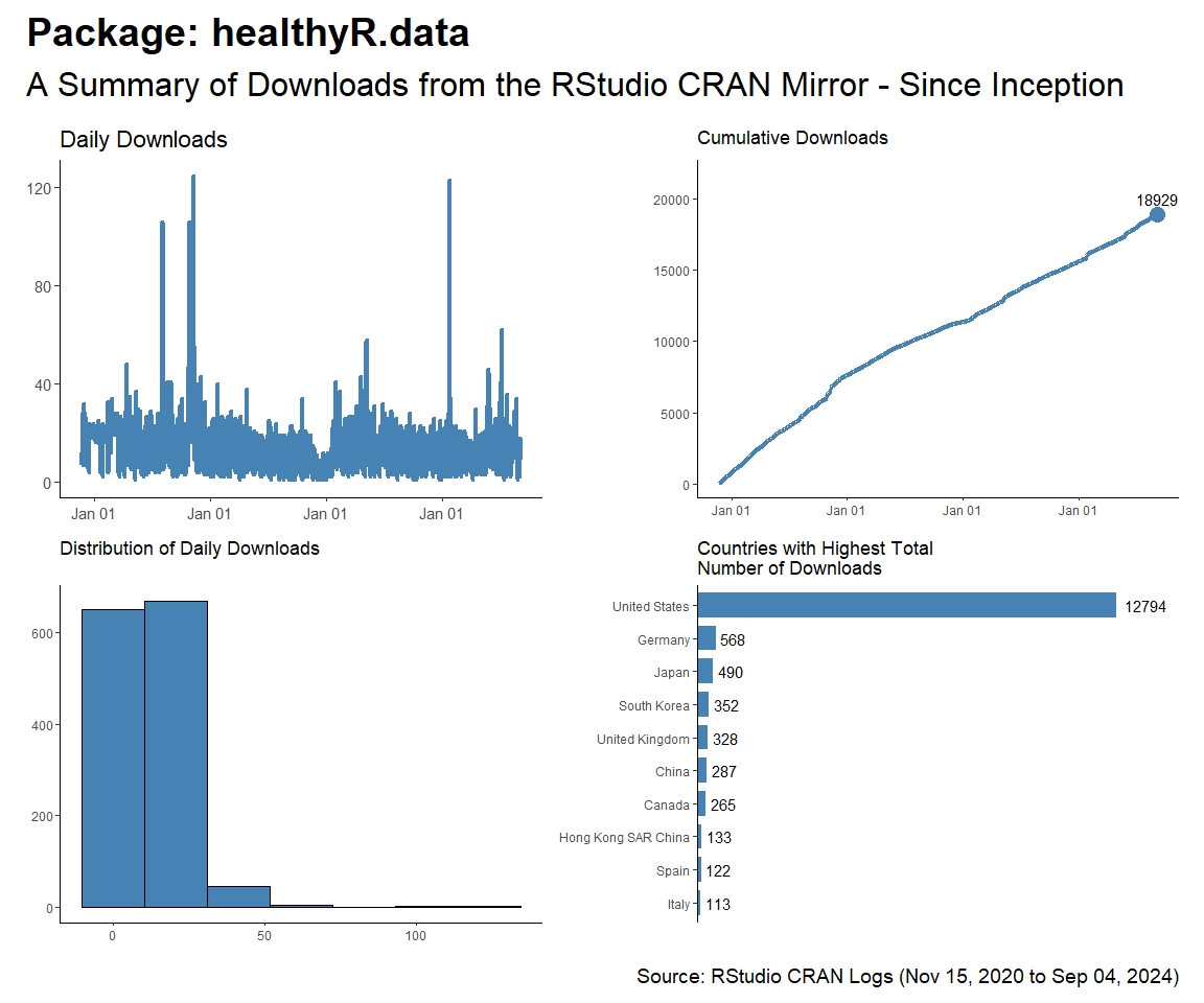
healthyR.data
start_date <- as.Date("2020-11-15")
pkg <- "healthyR.data"

daily_downloads <- compute_daily_downloads(
  downloads = total_downloads
  , pkg = pkg)
downloads_by_country <- compute_downloads_by_country(
  downloads = total_downloads
  , pkg = pkg)

p1 <- plot_daily_downloads(daily_downloads)
p2 <- plot_cumulative_downloads(daily_downloads)
p3 <- hist_daily_downloads(daily_downloads)
p4 <- plot_downloads_by_country(downloads_by_country)

f <- function(date) format(date, "%b %d, %Y")
patchwork_theme <- theme_classic(base_size = 24) +
  theme(
    plot.title   = element_text(face = "bold"),
    plot.caption = element_text(size = 14)
  )
p1 + p2 + p3 + p4 +
  plot_annotation(
    title    = glue::glue("Package: {pkg}"),
    subtitle = "A Summary of Downloads from the RStudio CRAN Mirror - Since Inception",
    caption  = glue::glue("Source: RStudio CRAN Logs ({f(start_date)} to {f(end_date)})"),
    theme    = patchwork_theme
  )
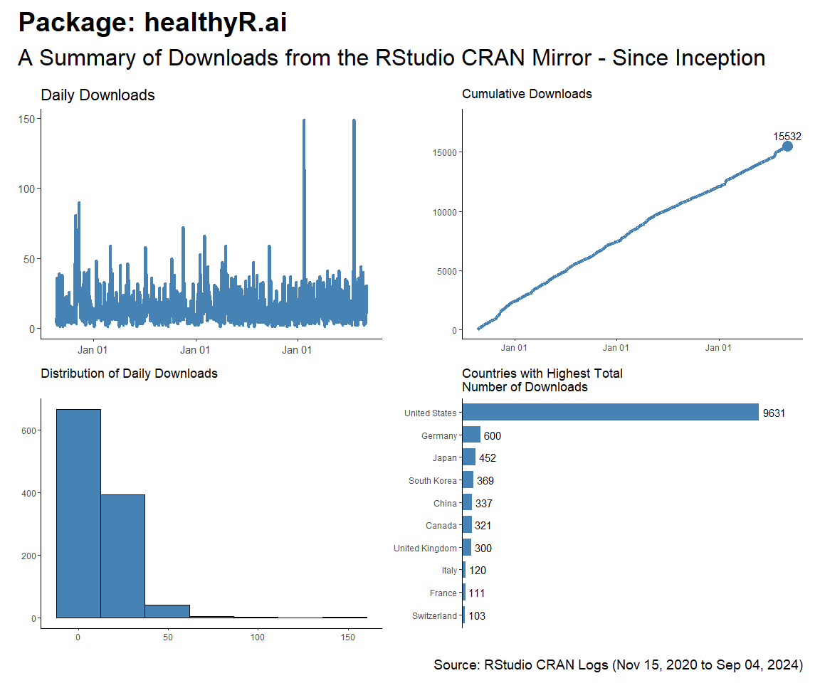
healthyR.ai
start_date <- as.Date("2020-11-15")
pkg <- "healthyR.ai"

daily_downloads <- compute_daily_downloads(
  downloads = total_downloads
  , pkg = pkg)
downloads_by_country <- compute_downloads_by_country(
  downloads = total_downloads
  , pkg = pkg)

p1 <- plot_daily_downloads(daily_downloads)
p2 <- plot_cumulative_downloads(daily_downloads)
p3 <- hist_daily_downloads(daily_downloads)
p4 <- plot_downloads_by_country(downloads_by_country)

f <- function(date) format(date, "%b %d, %Y")
patchwork_theme <- theme_classic(base_size = 24) +
  theme(
    plot.title   = element_text(face = "bold"),
    plot.caption = element_text(size = 14)
  )
p1 + p2 + p3 + p4 +
  plot_annotation(
    title    = glue::glue("Package: {pkg}"),
    subtitle = "A Summary of Downloads from the RStudio CRAN Mirror - Since Inception",
    caption  = glue::glue("Source: RStudio CRAN Logs ({f(start_date)} to {f(end_date)})"),
    theme    = patchwork_theme
  )
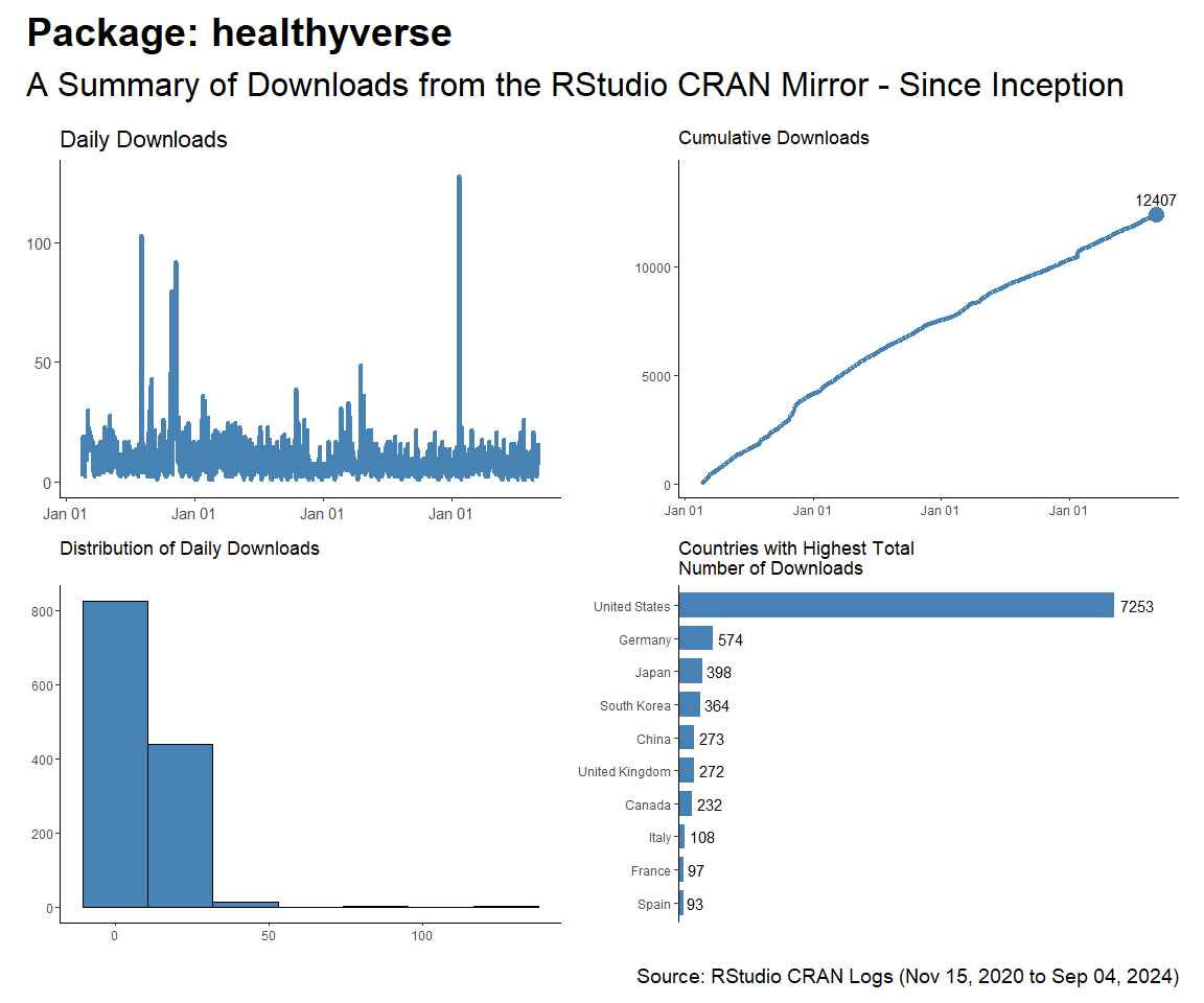
healthyverse
start_date <- as.Date("2020-11-15")
pkg <- "healthyverse"

daily_downloads <- compute_daily_downloads(
  downloads = total_downloads
  , pkg = pkg)
downloads_by_country <- compute_downloads_by_country(
  downloads = total_downloads
  , pkg = pkg)

p1 <- plot_daily_downloads(daily_downloads)
p2 <- plot_cumulative_downloads(daily_downloads)
p3 <- hist_daily_downloads(daily_downloads)
p4 <- plot_downloads_by_country(downloads_by_country)

f <- function(date) format(date, "%b %d, %Y")
patchwork_theme <- theme_classic(base_size = 24) +
  theme(
    plot.title   = element_text(face = "bold"),
    plot.caption = element_text(size = 14)
  )
p1 + p2 + p3 + p4 +
  plot_annotation(
    title    = glue::glue("Package: {pkg}"),
    subtitle = "A Summary of Downloads from the RStudio CRAN Mirror - Since Inception",
    caption  = glue::glue("Source: RStudio CRAN Logs ({f(start_date)} to {f(end_date)})"),
    theme    = patchwork_theme
  )
TidyDensity
start_date <- as.Date("2020-11-15")
pkg <- "TidyDensity"

daily_downloads <- compute_daily_downloads(
  downloads = total_downloads
  , pkg = pkg)
downloads_by_country <- compute_downloads_by_country(
  downloads = total_downloads
  , pkg = pkg)

p1 <- plot_daily_downloads(daily_downloads)
p2 <- plot_cumulative_downloads(daily_downloads)
p3 <- hist_daily_downloads(daily_downloads)
p4 <- plot_downloads_by_country(downloads_by_country)

f <- function(date) format(date, "%b %d, %Y")
patchwork_theme <- theme_classic(base_size = 24) +
  theme(
    plot.title   = element_text(face = "bold"),
    plot.caption = element_text(size = 14)
  )
p1 + p2 + p3 + p4 +
  plot_annotation(
    title    = glue::glue("Package: {pkg}"),
    subtitle = "A Summary of Downloads from the RStudio CRAN Mirror - Since Inception",
    caption  = glue::glue("Source: RStudio CRAN Logs ({f(start_date)} to {f(end_date)})"),
    theme    = patchwork_theme
  )

tidyAML
start_date <- as.Date("2023-02-13")
pkg <- "tidyAML"

daily_downloads <- compute_daily_downloads(
  downloads = total_downloads
  , pkg = pkg)
downloads_by_country <- compute_downloads_by_country(
  downloads = total_downloads
  , pkg = pkg)

p1 <- plot_daily_downloads(daily_downloads)
p2 <- plot_cumulative_downloads(daily_downloads)
p3 <- hist_daily_downloads(daily_downloads)
p4 <- plot_downloads_by_country(downloads_by_country)

f <- function(date) format(date, "%b %d, %Y")
patchwork_theme <- theme_classic(base_size = 24) +
  theme(
    plot.title   = element_text(face = "bold"),
    plot.caption = element_text(size = 14)
  )
p1 + p2 + p3 + p4 +
  plot_annotation(
    title    = glue::glue("Package: {pkg}"),
    subtitle = "A Summary of Downloads from the RStudio CRAN Mirror - Since Inception",
    caption  = glue::glue("Source: RStudio CRAN Logs ({f(start_date)} to {f(end_date)})"),
    theme    = patchwork_theme
  )

RandomWalker
start_date <- as.Date("2023-02-13")
pkg <- "RandomWalker"

daily_downloads <- compute_daily_downloads(
  downloads = total_downloads
  , pkg = pkg)
downloads_by_country <- compute_downloads_by_country(
  downloads = total_downloads
  , pkg = pkg)

p1 <- plot_daily_downloads(daily_downloads)
p2 <- plot_cumulative_downloads(daily_downloads)
p3 <- hist_daily_downloads(daily_downloads)
p4 <- plot_downloads_by_country(downloads_by_country)

f <- function(date) format(date, "%b %d, %Y")
patchwork_theme <- theme_classic(base_size = 24) +
  theme(
    plot.title   = element_text(face = "bold"),
    plot.caption = element_text(size = 14)
  )
p1 + p2 + p3 + p4 +
  plot_annotation(
    title    = glue::glue("Package: {pkg}"),
    subtitle = "A Summary of Downloads from the RStudio CRAN Mirror - Since Inception",
    caption  = glue::glue("Source: RStudio CRAN Logs ({f(start_date)} to {f(end_date)})"),
    theme    = patchwork_theme
  )
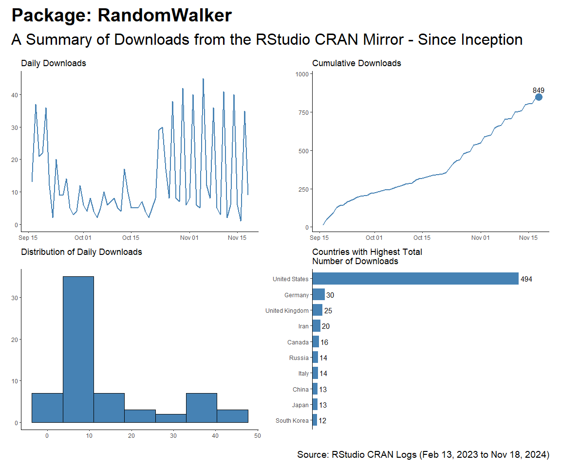
Table Data
Downloads by Package and Version
total_downloads %>%
  count(package, version) %>%
  tidyr::pivot_wider(
    id_cols       = version
    , names_from  = package
    , values_from = n
    , values_fill = 0
    ) %>%
  arrange(version) %>%
  kable()
| version | RandomWalker | TidyDensity | healthyR | healthyR.ai | healthyR.data | healthyR.ts | healthyverse | tidyAML |
|---|---|---|---|---|---|---|---|---|
| 0.0.1 | 0 | 1315 | 0 | 628 | 0 | 0 | 0 | 940 |
| 0.0.10 | 0 | 0 | 0 | 755 | 0 | 0 | 0 | 0 |
| 0.0.11 | 0 | 0 | 0 | 595 | 0 | 0 | 0 | 0 |
| 0.0.12 | 0 | 0 | 0 | 848 | 0 | 0 | 0 | 0 |
| 0.0.13 | 0 | 0 | 0 | 4174 | 0 | 0 | 0 | 0 |
| 0.0.13.tar.gz%20H | 0 | 0 | 0 | 5 | 0 | 0 | 0 | 0 |
| 0.0.2 | 0 | 0 | 0 | 1880 | 0 | 0 | 0 | 2045 |
| 0.0.3 | 0 | 0 | 0 | 642 | 0 | 0 | 0 | 733 |
| 0.0.4 | 0 | 0 | 0 | 725 | 0 | 0 | 0 | 976 |
| 0.0.5 | 0 | 0 | 0 | 1305 | 0 | 0 | 0 | 2940 |
| 0.0.6 | 0 | 0 | 0 | 2513 | 0 | 0 | 0 | 0 |
| 0.0.7 | 0 | 0 | 0 | 976 | 0 | 0 | 0 | 0 |
| 0.0.8 | 0 | 0 | 0 | 1102 | 0 | 0 | 0 | 0 |
| 0.0.9 | 0 | 0 | 0 | 893 | 0 | 0 | 0 | 0 |
| 0.1.0 | 425 | 0 | 519 | 1583 | 0 | 751 | 0 | 0 |
| 0.1.1 | 0 | 0 | 1567 | 0 | 0 | 2273 | 0 | 0 |
| 0.1.2 | 0 | 0 | 1790 | 0 | 0 | 1266 | 0 | 0 |
| 0.1.3 | 0 | 0 | 591 | 0 | 0 | 1383 | 0 | 0 |
| 0.1.4 | 0 | 0 | 641 | 0 | 0 | 951 | 0 | 0 |
| 0.1.5 | 0 | 0 | 1286 | 0 | 0 | 792 | 0 | 0 |
| 0.1.6 | 0 | 0 | 2493 | 0 | 0 | 528 | 0 | 0 |
| 0.1.7 | 0 | 0 | 1281 | 0 | 0 | 1522 | 0 | 0 |
| 0.1.8 | 0 | 0 | 2255 | 0 | 0 | 2240 | 0 | 0 |
| 0.1.9 | 0 | 0 | 1145 | 0 | 0 | 765 | 0 | 0 |
| 0.2.0 | 2929 | 0 | 2396 | 0 | 0 | 768 | 0 | 0 |
| 0.2.1 | 0 | 0 | 4637 | 0 | 0 | 582 | 0 | 0 |
| 0.2.1.tar.gz%20HT | 0 | 0 | 5 | 0 | 0 | 0 | 0 | 0 |
| 0.2.10 | 0 | 0 | 0 | 0 | 0 | 667 | 0 | 0 |
| 0.2.11 | 0 | 0 | 0 | 0 | 0 | 701 | 0 | 0 |
| 0.2.2 | 0 | 0 | 2373 | 0 | 0 | 812 | 0 | 0 |
| 0.2.2.tar.gz%20 | 0 | 0 | 0 | 0 | 0 | 10 | 0 | 0 |
| 0.2.3 | 0 | 0 | 0 | 0 | 0 | 816 | 0 | 0 |
| 0.2.4 | 0 | 0 | 0 | 0 | 0 | 439 | 0 | 0 |
| 0.2.5 | 0 | 0 | 0 | 0 | 0 | 735 | 0 | 0 |
| 0.2.6 | 0 | 0 | 0 | 0 | 0 | 596 | 0 | 0 |
| 0.2.7 | 0 | 0 | 0 | 0 | 0 | 984 | 0 | 0 |
| 0.2.8 | 0 | 0 | 0 | 0 | 0 | 2467 | 0 | 0 |
| 0.2.9 | 0 | 0 | 0 | 0 | 0 | 881 | 0 | 0 |
| 0.3.0 | 0 | 0 | 0 | 0 | 0 | 3051 | 0 | 0 |
| 0.3.0.tar.gz%20H | 0 | 0 | 0 | 0 | 0 | 5 | 0 | 0 |
| 0.3.1 | 0 | 0 | 0 | 0 | 0 | 1449 | 0 | 0 |
| 1.0.0 | 0 | 673 | 0 | 0 | 3154 | 0 | 2630 | 0 |
| 1.0.1 | 0 | 2061 | 0 | 0 | 10232 | 0 | 2435 | 0 |
| 1.0.2 | 0 | 0 | 0 | 0 | 2048 | 0 | 3826 | 0 |
| 1.0.3 | 0 | 0 | 0 | 0 | 3546 | 0 | 619 | 0 |
| 1.0.4 | 0 | 0 | 0 | 0 | 0 | 0 | 3603 | 0 |
| 1.1.0 | 0 | 712 | 0 | 0 | 627 | 0 | 1294 | 0 |
| 1.1.1 | 0 | 0 | 0 | 0 | 1249 | 0 | 0 | 0 |
| 1.2.0 | 0 | 794 | 0 | 0 | 668 | 0 | 0 | 0 |
| 1.2.1 | 0 | 610 | 0 | 0 | 0 | 0 | 0 | 0 |
| 1.2.2 | 0 | 825 | 0 | 0 | 0 | 0 | 0 | 0 |
| 1.2.3 | 0 | 857 | 0 | 0 | 0 | 0 | 0 | 0 |
| 1.2.4 | 0 | 3190 | 0 | 0 | 0 | 0 | 0 | 0 |
| 1.2.5 | 0 | 2052 | 0 | 0 | 0 | 0 | 0 | 0 |
| 1.2.6 | 0 | 1282 | 0 | 0 | 0 | 0 | 0 | 0 |
| 1.3.0 | 0 | 1823 | 0 | 0 | 0 | 0 | 0 | 0 |
| 1.4.0 | 0 | 1261 | 0 | 0 | 0 | 0 | 0 | 0 |
| 1.4.0.tar.gz%20H | 0 | 1 | 0 | 0 | 0 | 0 | 0 | 0 |
| 1.5.0 | 0 | 3944 | 0 | 0 | 0 | 0 | 0 | 0 |
| 1.5.0.tar.gz%20HT | 0 | 3 | 0 | 0 | 0 | 0 | 0 | 0 |
total_downloads %>%
  count(package, sort = TRUE) %>%
  tidyr::pivot_wider(
    names_from = package,
    values_from = n
  ) |>
  kable()
| healthyR.ts | healthyR | healthyR.data | TidyDensity | healthyR.ai | healthyverse | tidyAML | RandomWalker |
|---|---|---|---|---|---|---|---|
| 27434 | 22979 | 21524 | 21403 | 18624 | 14407 | 7634 | 3354 |
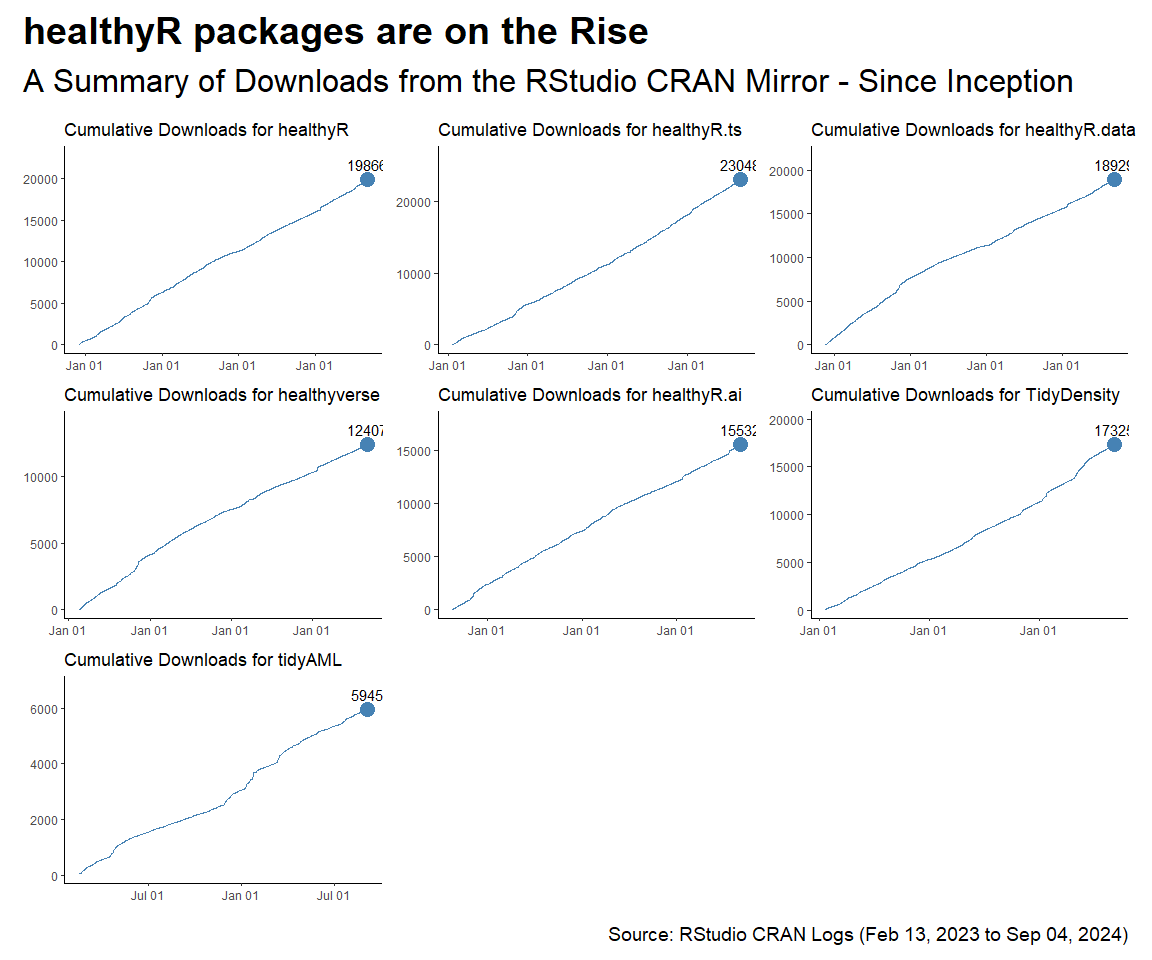
Cumulative Downloads by Package
p1 <- plot_cumulative_downloads_pkg(total_downloads, pkg = "healthyR")
p2 <- plot_cumulative_downloads_pkg(total_downloads, pkg = "healthyR.ts")
p3 <- plot_cumulative_downloads_pkg(total_downloads, pkg = "healthyR.data")
p4 <- plot_cumulative_downloads_pkg(total_downloads, pkg = "healthyverse")
p5 <- plot_cumulative_downloads_pkg(total_downloads, pkg = "healthyR.ai")
p6 <- plot_cumulative_downloads_pkg(total_downloads, pkg = "TidyDensity")
p7 <- plot_cumulative_downloads_pkg(total_downloads, pkg = "tidyAML")
p8 <- plot_cumulative_downloads_pkg(total_downloads, pkg = "RandomWalker")

f <- function(date) format(date, "%b %d, %Y")
patchwork_theme <- theme_classic(base_size = 24) +
  theme(
    plot.title   = element_text(face = "bold"),
    plot.caption = element_text(size = 14)
  )
p1 + p2 + p3 + p4 + p5 + p6 + p7 + p8 +
  plot_annotation(
    title    = "healthyR packages are on the Rise",
    subtitle = "A Summary of Downloads from the RStudio CRAN Mirror - Since Inception",
    caption  = glue::glue("Source: RStudio CRAN Logs ({f(start_date)} to {f(end_date)})"),
    theme    = patchwork_theme
  )
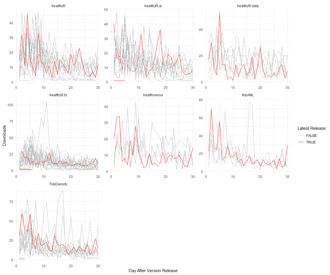
Thirty Day Run Post Release
pkg_rel <- readRDS("pkg_release_tbl.rds") |>
  # Filter out bad data, not sure why it occurrs.
  filter(
    date != "2024-05-29" &
      !(date == "2024-06-12" & package == "TidyDensity")
    ) |>
  arrange(date) |>
  group_by(package) |>
  mutate(rel_no = row_number()) |>
  ungroup()

thirty_day_runup_tbl <- total_downloads |>
  lazy_dt() |>
  select(date, package, version) |>
  group_by(date, package, version) |>
  summarise(dl_count = n()) |>
  ungroup() |>
  arrange(date) |>
  group_by(package, version) |>
  mutate(rec_no = row_number()) |>
  mutate(cum_dl = cumsum(dl_count)) |>
  filter(rec_no < 31) |>
  ungroup() |>
  mutate(pkg_ver = paste0(package, "-", version)) |>
  collect()

release_tbl <- left_join(
  x = thirty_day_runup_tbl,
  y = pkg_rel
) |>
  group_by(package) |>
  fill(release_record, .direction = "down") |>
  fill(rel_no, .direction = "down") |>
  mutate(
    release_record = as.factor(release_record),
    rel_no = as.factor(rel_no)
  ) |>
  ungroup()

latest_group_tbl <- release_tbl |>
  group_by(package) |>
  arrange(date, rec_no) |>
  mutate(group_no = as.numeric(rel_no)) |>
  filter(group_no == max(group_no)) |>
  ungroup()

joined_tbl <- left_join(
  x = thirty_day_runup_tbl,
  y = latest_group_tbl
  ) |>
  mutate(group_no = ifelse(is.na(group_no), FALSE, TRUE))

joined_tbl |>
  ggplot(aes(x = rec_no, y = dl_count, group = as.factor(pkg_ver))) +
  facet_wrap(~ package, scales = "free", ncol = 3) +
  geom_line(aes(col = group_no)) +
  scale_color_manual(values = c("FALSE" = "grey", "TRUE" = "red")) +
  theme_minimal() +
  labs(
    y = "Downloads",
    x = "Day After Version Release",
    col = "Latest Release"
  )
joined_tbl |>
  ggplot(aes(x = rec_no, y = cum_dl, group = as.factor(pkg_ver))) +
  facet_wrap(~ package, scales = "free", ncol = 3) +
  geom_line(aes(col = group_no)) +
  scale_color_manual(values = c("FALSE" = "grey", "TRUE" = "red")) +
  theme_minimal() +
  labs(
    y = "Downloads",
    x = "Day After Version Release",
    col = "Latest Release"
  )
