Introduction

Welcome to the world of data visualization in R! In this blog post, we will explore the abline() function, a versatile tool that allows you to add straight lines to your plots effortlessly. Whether you’re a beginner or an experienced R programmer, mastering abline() will empower you to create more informative and visually appealing graphs. So, let’s dive in!

Understanding abline()

The abline() function in R enables you to draw straight lines on a plot, making it a powerful tool for visualizing relationships, trends, and patterns in your data. It accepts several arguments: The a and b parameters specify the intercept and slope of the line, respectively. The h and v parameters specify the y-value and x-value for horizontal and vertical lines, respectively. The … parameters can be used to specify other graphical parameters, such as the line type and width.

Syntax

The basic syntax of the abline() function is as follows:

abline(
  a = NULL, 
  b = NULL, 
  v = NULL, 
  reg = NULL,
  coef = NULL, 
  untf = FALSE, 
  ...)

Examples

Example 1. Simple Linear Regression Line:

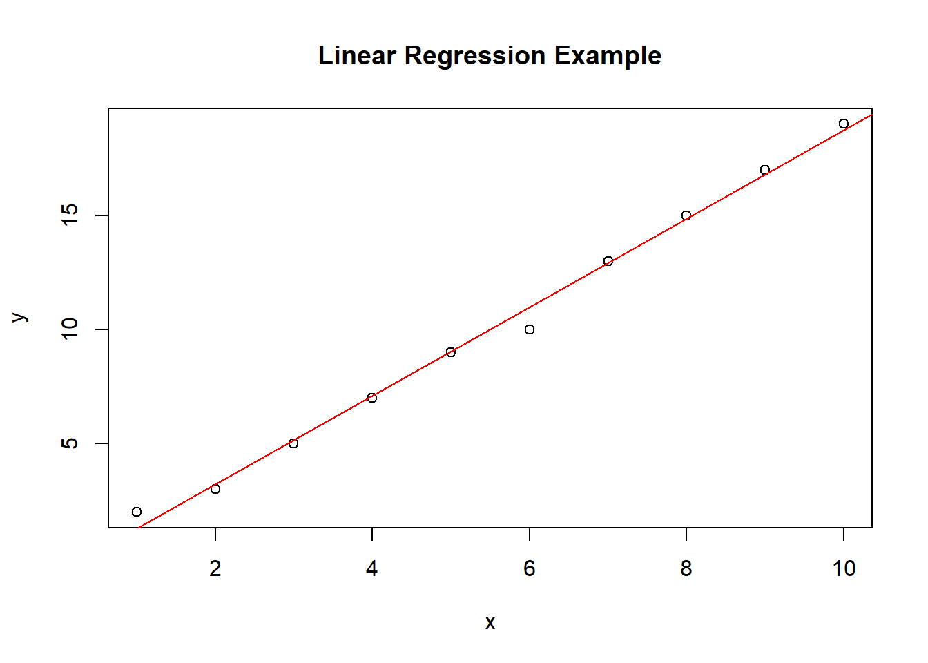
Let’s start with a classic example of drawing a linear regression line on a scatter plot. Consider the following data:

x <- 1:10
y <- c(2, 3, 5, 7, 9, 10, 13, 15, 17, 19)

To visualize the relationship between x and y, we can plot the points and add a regression line using abline():

plot(x, y, main = "Linear Regression Example", xlab = "x", ylab = "y")
abline(lm(y ~ x), col = "red")

Examle 2. Custom Slope and Intercept

The abline() function allows you to specify custom slope and intercept values. Suppose you have a dataset where y increases by 3 for every unit increase in x. We can draw a line with a slope of 3 and an intercept of 0 using the following code:

plot(x, y, main = "Custom Slope and Intercept", xlab = "x", ylab = "y")
abline(a = 0, b = 3, col = "blue")

Example 3. Vertical and Horizontal Lines:

abline() isn’t limited to just diagonal lines; you can also draw vertical and horizontal lines. For instance, let’s draw a vertical line at x = 5 and a horizontal line at y = 12:

plot(x, y, main = "Vertical and Horizontal Lines", xlab = "x", ylab = "y")
abline(v = 5, col = "green") # Vertical line
abline(h = 12, col = "orange") # Horizontal line

Encouragement to Try It Yourself

Now that you’ve seen a few examples of what the abline() function can do, I encourage you to unleash your creativity and explore its full potential. Experiment with different datasets, slopes, intercepts, and line styles. The more you practice, the more comfortable you will become with this powerful visualization tool.

Conclusion

In this blog post, we delved into the abline() function in R, exploring its capabilities for adding straight lines to plots. We covered simple linear regression lines, custom slopes and intercepts, as well as vertical and horizontal lines. Armed with this knowledge, you can enhance your data visualizations, making them more informative and engaging. So, go ahead, give abline() a try, and unlock a whole new world of possibilities in R programming! Happy coding!