Introduction

Hey there, fellow R enthusiasts! Today, let’s embark on a fascinating journey into the realm of piecewise regression using R. If you’ve ever wondered how to uncover hidden trends and breakpoints in your data, you’re in for a treat. Buckle up, and let’s dive into the world of piecewise regression!

Piecewise Regression

Piecewise regression is a powerful technique that allows us to model distinct segments of a dataset with different linear relationships. It’s like fitting multiple straight lines to capture the nuances of different regions in your data. So, grab your virtual lab coat, and let’s get started.

Example

Step 1: Load Your Data and Libraries

# Install and load necessary packages
# install.packages("segmented")
library(segmented)

# Sample data
set.seed(123)
x <- 1:100
y <- 2 + 1.5 * pmax(x - 35, 0) - 1.5 * pmax(x - 70, 0) + rnorm(100)

# Combine data
data <- data.frame(x, y)

Step 2: Explore Your Data

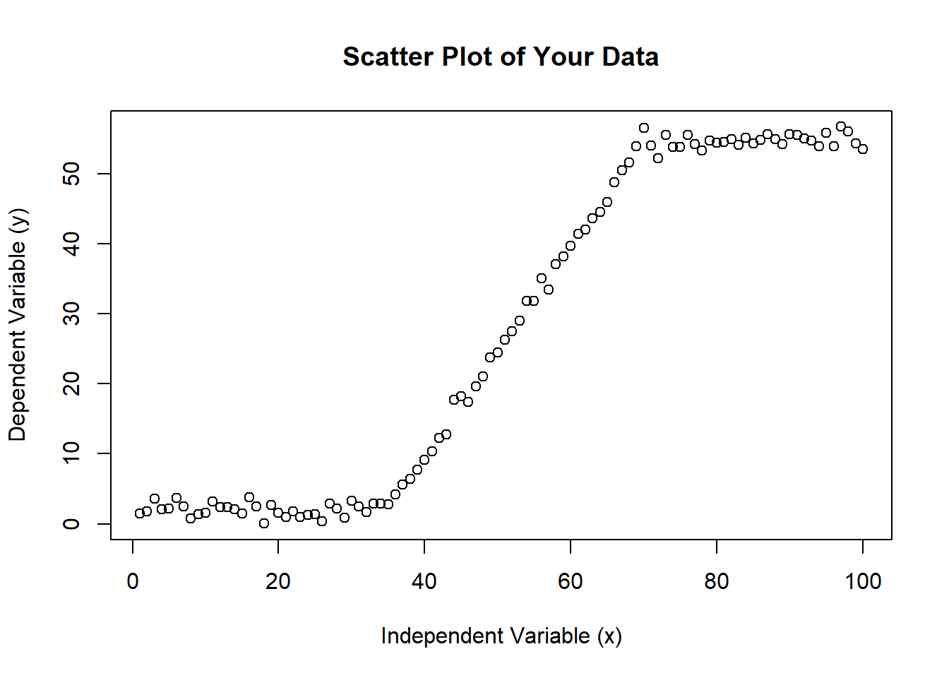
Before diving into the regression, let’s take a peek at our data. Visualizing the data often provides insights into potential breakpoints.

# Scatter plot to visualize the data
plot(
  data$x, data$y, 
  main = "Scatter Plot of Your Data",
  xlab = "Independent Variable (x)", 
  ylab = "Dependent Variable (y)")

Step 3: Perform Piecewise Regression

Now, the exciting part! Let’s fit our piecewise regression model using the segmented package.

# Fit the piecewise regression model
model <- lm(y ~ x, data = data)
segmented_model <- segmented(model, seg.Z = ~x)

Step 4: Visualize the Results:

To truly understand the magic happening, let’s visualize the fitted model and residuals.

seg_preds <- predict(segmented_model)
seg_res <- y - seg_preds

# Plot the original data with the fitted model
plot(
  data$x, data$y,
  main = "Piecewise Regression Fit",
  xlab = "Independent Variable (x)",
  ylab = "Dependent Variable (y)",
  col = "blue"
)
lines(data$x, seg_preds,col = "red", lwd = 2)

# Plot residuals
# Plot the residuals for each segment
plot(x, seg_res, main = "Residuals")
abline(h = 0, col = "red")

Step 5: Interpret the Breakpoints:

Inspecting the segmented model will reveal the breakpoints and the corresponding regression lines. It’s like deciphering the story your data is trying to tell.

# View breakpoints and coefficients
summary(segmented_model)


    ***Regression Model with Segmented Relationship(s)***

Call: 
segmented.lm(obj = model, seg.Z = ~x)

Estimated Break-Point(s):
          Est. St.Err
psi1.x 24.757  3.074

Coefficients of the linear terms:
            Estimate Std. Error t value Pr(>|t|)
(Intercept)  2.49825    2.55867   0.976    0.331
x           -0.04055    0.17907  -0.226    0.821
U1.x         0.93569    0.18186   5.145       NA

Residual standard error: 6.073 on 96 degrees of freedom
Multiple R-Squared: 0.9333,  Adjusted R-squared: 0.9312 

Boot restarting based on 6 samples. Last fit:
Convergence attained in 2 iterations (rel. change 2.9855e-12)

Step 6: Encourage Exploration:

Now that you’ve conquered piecewise regression, encourage your fellow data explorers to try it themselves. Challenge them to apply this technique to their datasets and share their insights.

Conclusion

Congratulations, you’ve just unlocked the power of piecewise regression in R! By visualizing data, fitting models, and exploring breakpoints, you’ve gained a valuable tool for understanding complex relationships. Keep coding, keep exploring, and stay curious!

Happy coding, and may your data always reveal its secrets!

Steven P. Sanderson II, MPH