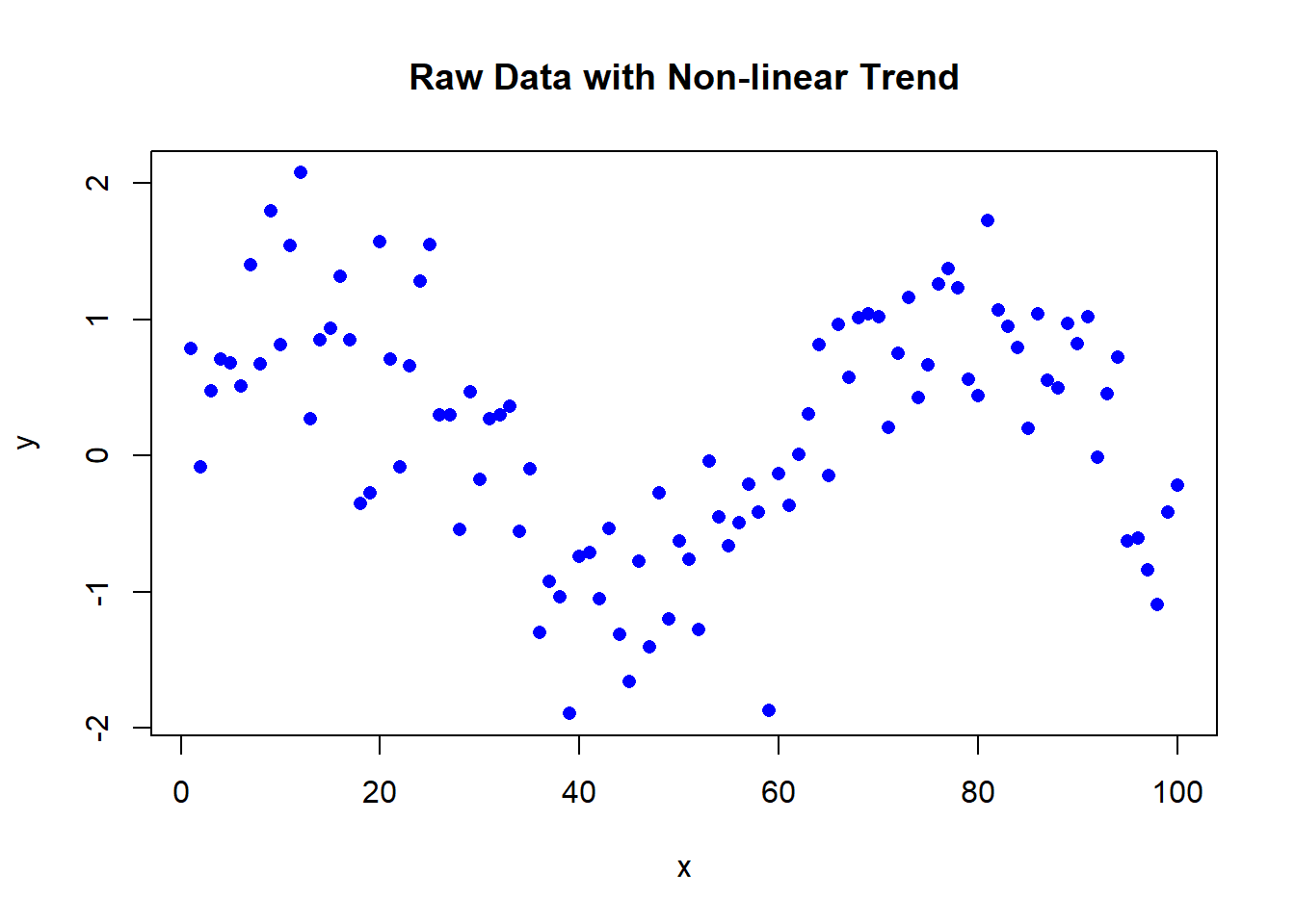
# Set seed for reproducibility
set.seed(42)

# Generate data
x <- seq(1, 100, by = 1)
y <- sin(x/10) + rnorm(100, sd = 0.5)

# Plot the raw data
plot(x, y, main = "Raw Data with Non-linear Trend", col = "blue", pch = 16)
Steven P. Sanderson II, MPH
January 2, 2024
Hey fellow R enthusiasts! Today, let’s dive into the fascinating world of Lowess smoothing and learn how to harness its power for creating smooth visualizations of your data. Whether you’re new to R or a seasoned pro, this step-by-step guide will walk you through the process of performing Lowess smoothing, generating data, visualizing the model, and comparing different models with varying smoother spans.
Locally Weighted Scatterplot Smoothing, or Lowess, is a powerful technique for capturing trends in noisy data. It’s particularly useful when dealing with datasets that exhibit complex patterns that might be missed by other methods. So, let’s get our hands dirty and start coding!
Before we can smooth anything, we need some data to work with. Let’s create a synthetic dataset using the rnorm function and introduce a non-linear trend:
Now that we have our data, let’s apply Lowess smoothing using the lowess function:
To better understand our smoothed model, let’s visualize the fitted values along with the residuals:
# Get fitted values and residuals
fitted_values <- smoothed_data$y
residuals <- y - fitted_values

# Plot the model
plot(x, fitted_values, main = "Lowess Smoothed Model with Residuals", col = "red", type = "l", lwd = 2)
points(x, residuals, col = "green", pch = 16)
legend("topleft", legend = c("Smoothed Model", "Residuals"), col = c("red", "green"), lwd = 2)
Now, let’s take our Lowess smoothing to the next level by experimenting with different smoother spans. We’ll create three models with varying spans and visualize the differences:
# Generate three smoothed models with different spans
model_1 <- lowess(x, y, f = 0.2)
model_2 <- lowess(x, y, f = 0.5)
model_3 <- lowess(x, y, f = 0.8)

# Plot the original data
plot(x, y, main = "Comparison of Lowess Models", col = "blue", pch = 16)

# Plot the smoothed models
lines(model_1, col = "red", lty = 2, lwd = 2)
lines(model_2, col = "green", lty = 3, lwd = 2)
lines(model_3, col = "purple", lty = 4, lwd = 2)

# Add a legend
legend("bottomleft", legend = c("Raw Data", "Model 1", "Model 2", "Model 3"), col = c("blue", "red", "green", "purple"), lwd = 2)
And there you have it – a quick on performing Lowess smoothing in R! Feel free to tweak the parameters and explore the nuances of different models. Happy coding!