Introduction

Data normalization is a crucial preprocessing step in data analysis and machine learning workflows. It helps in standardizing the scale of numeric features, ensuring fair treatment to all variables regardless of their magnitude. In this tutorial, we’ll explore how to normalize data in R using practical examples and step-by-step explanations.

Example

Step 1: Prepare Your Data

For demonstration purposes, let’s create a sample dataset. Suppose we have a dataset called my_data with three numeric variables: age, income, and education.

set.seed(42) # reproducible
# Create a sample dataset
my_data <- data.frame(
  age = trunc(runif(250, 25, 65)),
  income = round(rlnorm(250, log(71000))),
  education = trunc(runif(250, 12, 20))
)

Step 2: Normalize the Data

Now, let’s normalize the numeric variables in our dataset. We’ll use the scale() function to standardize each variable to have a mean of 0 and a standard deviation of 1.

# Normalize the data
normalized_data <- data.frame(
  age_normalized = scale(my_data$age),
  income_normalized = scale(my_data$income),
  education_normalized = scale(my_data$education)
)

Step 3: Understand the Normalized Data

After normalization, each variable will have a mean of approximately 0 and a standard deviation of 1. This ensures that all variables are on the same scale, making them comparable and suitable for various analytical techniques.

# View the normalized data
head(normalized_data)

  age_normalized income_normalized education_normalized
1     1.38435717        -0.5141139           -0.9663645
2     1.47019281        -0.5829717           -1.3865230
3    -0.76153378        -0.8385455           -0.1260475
4     1.12685026        -0.7375278           -0.9663645
5     0.44016515        -0.1738354           -0.9663645
6     0.01098696         0.1804609           -0.5462060

Step 4: Interpret the Results

In the output, you’ll notice that each variable now has its normalized counterpart. For example:

age_normalized represents the standardized values of the age variable.
income_normalized represents the standardized values of the income variable.
education_normalized represents the standardized values of the education variable.

Step 5: Visualize the Normalized Data (Optional)

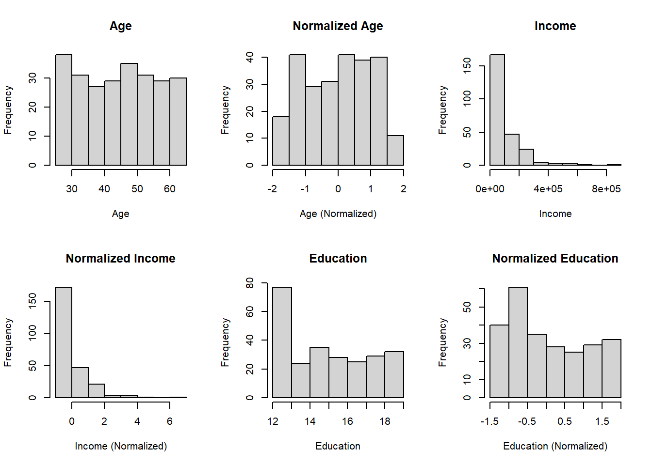
To gain a better understanding of the normalization process, you can visualize the distribution of the original and normalized variables using histograms or density plots.

# Visualize the original and normalized data (Optional)
par(mfrow = c(2, 3)) # Arrange plots in a 2x3 grid
hist(my_data$age, main = "Age", xlab = "Age")
hist(normalized_data$age_normalized, main = "Normalized Age", xlab = "Age (Normalized)")

hist(my_data$income, main = "Income", xlab = "Income")
hist(normalized_data$income_normalized, main = "Normalized Income", xlab = "Income (Normalized)")

hist(my_data$education, main = "Education", xlab = "Education")
hist(normalized_data$education_normalized, main = "Normalized Education", xlab = "Education (Normalized)")

Conclusion

Congratulations! You’ve successfully normalized your data in R. By standardizing the scale of numeric variables, you’ve prepared your data for further analysis, ensuring fair treatment to all variables. Feel free to explore more advanced techniques or apply normalization to your own datasets.

I encourage you to try this process on your own datasets and experiment with different normalization techniques. Happy analyzing!