Introduction

Hello R users! Today, let’s explore the latest addition to the TidyDensity package: util_chisquare_param_estimate(). This function is designed to estimate parameters for a Chi-square distribution from your data, providing valuable insights into the underlying distribution characteristics.

Understanding the Purpose

The util_chisquare_param_estimate() function is a powerful tool for analyzing data that conforms to a Chi-square distribution. It utilizes maximum likelihood estimation (MLE) to infer the degrees of freedom (dof) and non-centrality parameter (ncp) of the Chi-square distribution based on your input vector.

Getting Started

To begin, let’s generate a dataset that conforms to a Chi-square distribution:

library(TidyDensity)

# Generate Chi-square distributed data
set.seed(123)
data <- rchisq(250, 10, 2)

# Call util_chisquare_param_estimate()
result <- util_chisquare_param_estimate(data)

By default, the function will automatically generate empirical distribution data if .auto_gen_empirical is set to TRUE. This means you’ll not only get the Chi-square parameters but also a combined table of empirical and Chi-square distribution data.

Exploring the Output

Let’s unpack what the function returns:

dist_type: Identifies the type of distribution, which will be “Chisquare” for this analysis.
samp_size: Indicates the sample size, i.e., the number of data points in your vector .x.
min, max, mean: Basic statistics summarizing your data.
dof: The estimated degrees of freedom for the Chi-square distribution.
ncp: The estimated non-centrality parameter for the Chi-square distribution.

This comprehensive output allows you to gain deeper insights into your data’s distribution characteristics, particularly when the Chi-square distribution is a potential model.

Let’s now take a look at the output itself.

library(dplyr)

result$combined_data_tbl |>
  head(5) |>
  glimpse()

Rows: 5
Columns: 8
$ sim_number <fct> 1, 1, 1, 1, 1
$ x          <int> 1, 2, 3, 4, 5
$ y          <dbl> 12.716908, 17.334453, 11.913559, 15.252845, 7.208524
$ dx         <dbl> -2.100590, -1.952295, -1.803999, -1.655704, -1.507408
$ dy         <dbl> 2.741444e-05, 3.676673e-05, 4.930757e-05, 6.515313e-05, 8.6…
$ p          <dbl> 0.640, 0.848, 0.576, 0.744, 0.204
$ q          <dbl> 2.765968, 3.205658, 3.297085, 3.567437, 3.869764
$ dist_type  <fct> "Empirical", "Empirical", "Empirical", "Empirical", "Empiri…

result$combined_data_tbl |>
  tidy_distribution_summary_tbl(dist_type) |>
  glimpse()

Rows: 2
Columns: 13
$ dist_type  <fct> "Empirical", "Chisquare c(9.961, 1.979)"
$ mean_val   <dbl> 11.95263, 12.04686
$ median_val <dbl> 10.79615, 11.48777
$ std_val    <dbl> 5.438087, 5.349567
$ min_val    <dbl> 2.765968, 1.922223
$ max_val    <dbl> 29.95844, 30.43480
$ skewness   <dbl> 0.9344797, 0.6903444
$ kurtosis   <dbl> 3.790972, 3.243122
$ range      <dbl> 27.19248, 28.51258
$ iqr        <dbl> 7.469292, 7.282262
$ variance   <dbl> 29.57279, 28.61787
$ ci_low     <dbl> 4.010739, 3.997601
$ ci_high    <dbl> 26.33689, 23.60014

Behind the Scenes: MLE Optimization

Under the hood, the function leverages MLE through the optim() function to estimate the Chi-square parameters. It minimizes the negative log-likelihood function to obtain the best-fitting degrees of freedom (dof) and non-centrality parameter (ncp) for your data.

Initial values for the optimization are intelligently set based on your data’s sample variance and mean, ensuring a robust estimation process.

Visualizing the Results

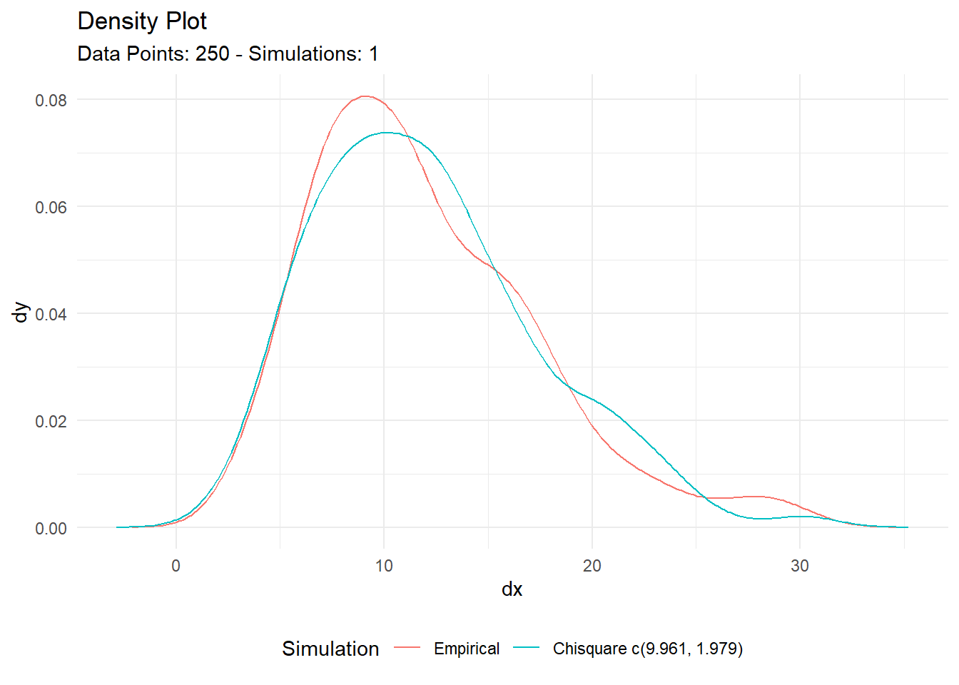
One of the strengths of TidyDensity is its seamless integration with visualization tools like ggplot2. With the combined output from util_chisquare_param_estimate(), you can easily create insightful plots that compare the empirical distribution with the estimated Chi-square distribution.

result$combined_data_tbl |>
  tidy_combined_autoplot()

This example demonstrates how you can visualize the empirical data overlaid with the fitted Chi-square distribution, providing a clear representation of your dataset’s fit to the model.

Conclusion

In summary, util_chisquare_param_estimate() from TidyDensity is a versatile tool for estimating Chi-square distribution parameters from your data. Whether you’re exploring the underlying distribution of your dataset or conducting statistical inference, this function equips you with the necessary tools to gain valuable insights.

If you haven’t already, give it a try and let us know how you’re using TidyDensity to enhance your data analysis workflows! Stay tuned for more updates and insights from the world of R programming. Happy coding!