library(healthyR.ts)
library(tidyverse)
library(timetk)
library(rsample)Introduction
Hello everyone,
I’m excited to give you an overview of healthyR.ts, an R package designed to simplify and enhance your time series analysis experience. Just like my healthyR package, it is designed to be user friendly.
What is healthyR.ts?
healthyR.ts is a robust package that integrates seamlessly with your existing R environment, providing a comprehensive toolkit for time series analysis. Its goal is to streamline the workflow, allowing you to focus on insights rather than the intricacies of implementation.
Key Features
1. Versatile Functionality
healthyR.ts comes packed with functions to handle various aspects of time series analysis, from basic preprocessing to advanced modeling and forecasting. Whether you need to decompose your series, detect anomalies, or fit complex models, healthyR.ts has got you covered.
2. User-Friendly Interface
The package is designed with usability in mind. Functions are well-documented and intuitive, making it easier for users at all levels to implement sophisticated time series techniques. You can find a comprehensive list of functions and their detailed descriptions in the Reference Section.
3. Seamless Integration
healthyR.ts integrates smoothly with other popular R packages, enhancing its utility and flexibility. This allows you to leverage the strengths of multiple tools within a single workflow, optimizing your analysis process.
Latest Updates
We’re continually working to improve healthyR.ts, adding new features and refining existing ones based on user feedback and advancements in the field. Check out the Latest News Section to stay updated with the most recent changes and enhancements.
Installation
You can install the released version of healthyR.ts from CRAN with:
install.packages("healthyR.ts")And the development version from GitHub with:
# install.packages("devtools")
devtools::install_github("spsanderson/healthyR.ts")
Getting Started
Let’s take a quick look at how you can use healthyR.ts for a variety of problems. Here’s a simple example to get you started:
First, let’s load in our libraries:
Now, let’s generate some sample data:
# Generate
set.seed(123)
df <- ts_random_walk()
Let’s take a look at our data:
glimpse(df)Rows: 10,000
Columns: 4
$ run <dbl> 1, 1, 1, 1, 1, 1, 1, 1, 1, 1, 1, 1, 1, 1, 1, 1, 1, 1, 1, 1, 1, 1…
$ x <dbl> 1, 2, 3, 4, 5, 6, 7, 8, 9, 10, 11, 12, 13, 14, 15, 16, 17, 18, 1…
$ y <dbl> -0.056047565, -0.023017749, 0.155870831, 0.007050839, 0.01292877…
$ cum_y <dbl> 943.9524, 922.2248, 1065.9727, 1073.4887, 1087.3676, 1273.8582, …Now let’s review the function we just used. Here is some information about the ts_random_walk function:
Syntax:
ts_random_walk(
  .mean = 0,
  .sd = 0.1,
  .num_walks = 100,
  .periods = 100,
  .initial_value = 1000
)
Arguments:
.mean: The desired mean of the random walks.sd: The standard deviation of the random walks.num_walks: The number of random walks you want generated.periods: The length of the random walk(s) you want generated.initial_value: The initial value where the random walks should start
Visualize
Now, let’s visualize our data:
df |>
   ggplot(
       mapping = aes(
           x = x
           , y = cum_y
           , color = factor(run)
           , group = factor(run)
        )
    ) +
    geom_line(alpha = 0.8) +
    ts_random_walk_ggplot_layers(df)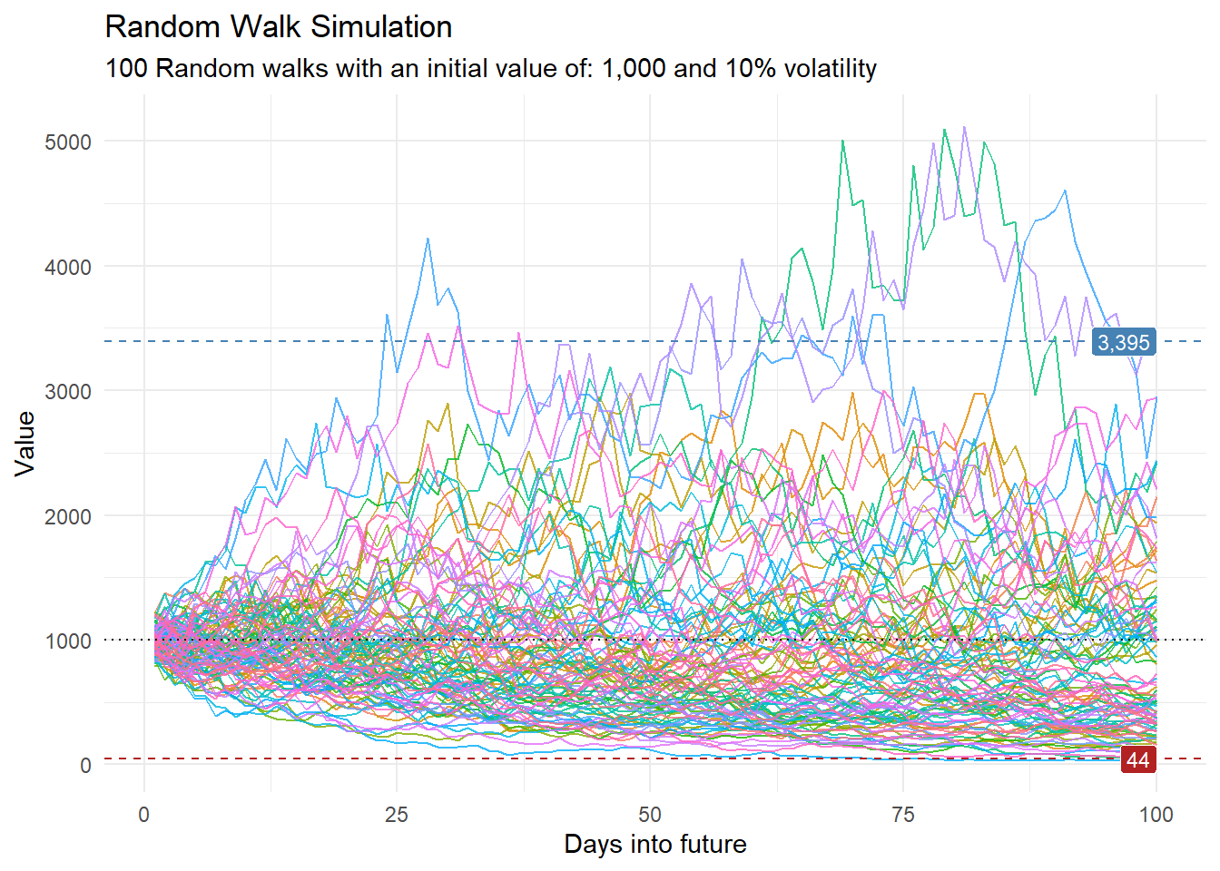
library(dplyr)
library(ggplot2)

df |>
    group_by(x) |>
    summarise(
        min_y = min(cum_y),
        max_y = max(cum_y)
    ) |>
    ggplot(
        aes(x = x)
    ) +
    geom_line(aes(y = max_y), color = "steelblue") +
    geom_line(aes(y = min_y), color = "firebrick") +
    geom_ribbon(aes(ymin = min_y, ymax = max_y), alpha = 0.2) +
    ts_random_walk_ggplot_layers(df)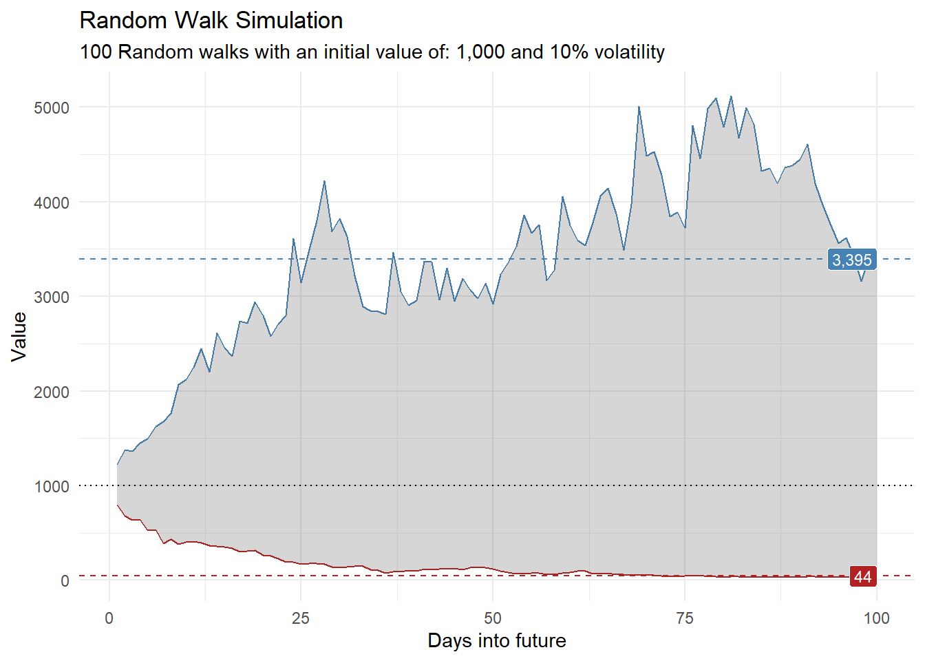
Now we have just gone over how to use a function to generate a simple random walk, this is only scratching the surface of what this package can do. I am going to go over a few more examples and try to break things up into sections.
Examples
Generating Functions
We have already gone over how to generate a simple random walk, but there are other functions that can be used to generate data. Here are examples:
ts_brownian_motion
# Generate
set.seed(123)
bm <- ts_brownian_motion()
glimpse(bm)
Rows: 1,010
Columns: 3
$ sim_number <fct> sim_number 1, sim_number 2, sim_number 3, sim_number 4, sim…
$ t <int> 1, 1, 1, 1, 1, 1, 1, 1, 1, 1, 2, 2, 2, 2, 2, 2, 2, 2, 2, 2,…
$ y <dbl> 0.00000000, 0.00000000, 0.00000000, 0.00000000, 0.00000000,…bm |>
ts_brownian_motion_plot(
.date_col = t,
.value_col = y,
.interactive = TRUE
)ts_geometric_brownian_motion
gm <- ts_geometric_brownian_motion()
glimpse(gm)
Rows: 2,600
Columns: 3
$ sim_number <fct> sim_number 1, sim_number 2, sim_number 3, sim_number 4, sim…
$ t <int> 1, 1, 1, 1, 1, 1, 1, 1, 1, 1, 1, 1, 1, 1, 1, 1, 1, 1, 1, 1,…
$ y <dbl> 100, 100, 100, 100, 100, 100, 100, 100, 100, 100, 100, 100,…gm |>
ts_brownian_motion_plot(
.date_col = t,
.value_col = y,
.interactive = TRUE
)Plotting Functions
The package also includes a variety of plotting functions to help you visualize your data. Here are a few examples:
ts_vva_plot
# Generate
set.seed(123)
df <- ts_random_walk(.num_walks = 1, .periods = 100) |>
  filter(run == 1)
glimpse(df)
Rows: 200
Columns: 4
$ run <dbl> 1, 1, 1, 1, 1, 1, 1, 1, 1, 1, 1, 1, 1, 1, 1, 1, 1, 1, 1, 1, 1, 1…
$ x <dbl> 1, 2, 3, 4, 5, 6, 7, 8, 9, 10, 11, 12, 13, 14, 15, 16, 17, 18, 1…
$ y <dbl> -0.056047565, -0.023017749, 0.155870831, 0.007050839, 0.01292877…
$ cum_y <dbl> 943.9524, 922.2248, 1065.9727, 1073.4887, 1087.3676, 1273.8582, …ts_vva_plot(
.data = df,
.date_col = x,
.value_col = cum_y
)$data
$data$augmented_data_tbl
# A tibble: 600 × 3
x name value
<dbl> <fct> <dbl>
1 1 Cum_y 944.
2 1 Velocity NA
3 1 Acceleration NA
4 2 Cum_y 922.
5 2 Velocity -21.7
6 2 Acceleration NA
7 3 Cum_y 1066.
8 3 Velocity 144.
9 3 Acceleration 165.
10 4 Cum_y 1073.
# ℹ 590 more rows
$plots
$plots$static_plotWarning: Removed 2 rows containing missing values or values outside the scale range
(`geom_line()`).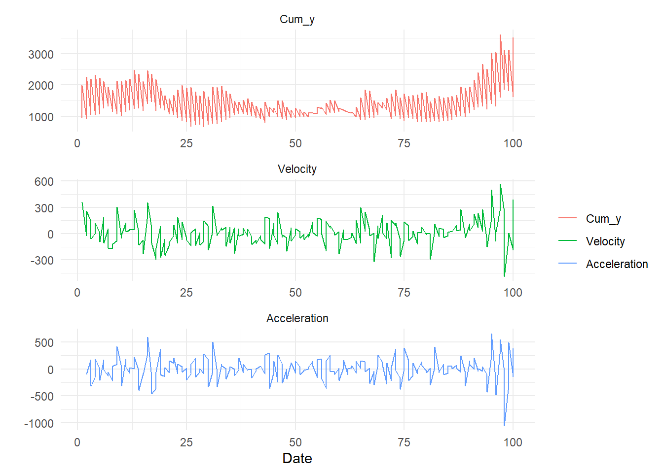
$plots$interactive_plotFiltering Functions
ts_compare_data
Compare data over time periods:
data_tbl <- ts_to_tbl(AirPassengers) |>
  select(-index)

ts_compare_data(
  .data           = data_tbl
  , .date_col     = date_col
  , .start_date   = "1955-01-01"
  , .end_date     = "1955-12-31"
  , .periods_back = "2 years"
  ) |>
  summarise_by_time(
    .date_var = date_col
    , .by     = "year"
    , visits  = sum(value)
  )
# A tibble: 2 × 2
date_col visits
<date> <dbl>
1 1953-01-01 2700
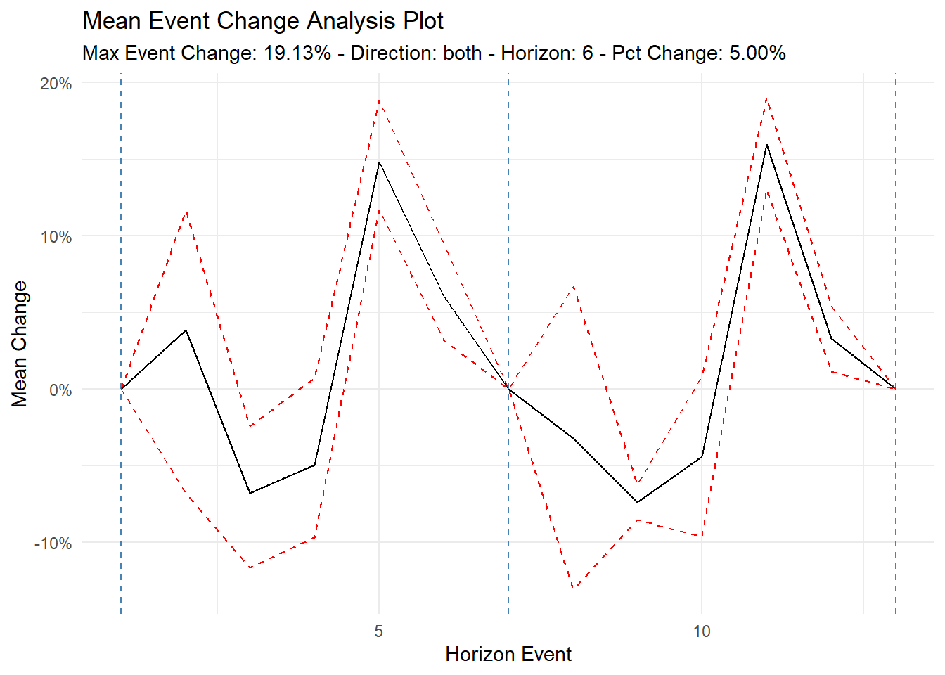
2 1955-01-01 3408ts_time_event_analysis_tbl
tst <- ts_time_event_analysis_tbl(
  data_tbl,
  date_col,
  value,
  .direction = "both",
  .horizon = 6
)

tst |>
  ts_event_analysis_plot(
  .plot_type = "mean",
  .plot_ci = TRUE,
  .interactive = FALSE
)
Simulator
ts_arima_simiulator
Simulate an arima model and visualize the results:
output <- ts_arima_simulator()
output$plots$static_plot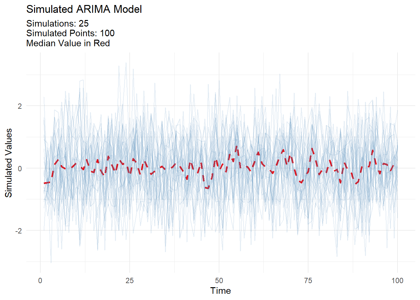
Auto Workflowset Generators
Want to create an automatic workflow set of data? Got you covered
ts_wfs_
splits <- time_series_split(
   data_tbl
  , date_col
  , assess = 12
  , skip = 3
  , cumulative = TRUE
)

rec_objs <- ts_auto_recipe(
 .data = training(splits)
 , .date_col = date_col
 , .pred_col = value
)

wf_sets <- ts_wfs_arima_boost("all_engines", rec_objs)
wf_sets
# A workflow set/tibble: 8 × 4
wflow_id info option result
<chr> <list> <list> <list>
1 rec_base_arima_boost_1 <tibble [1 × 4]> <opts[0]> <list [0]>
2 rec_base_arima_boost_2 <tibble [1 × 4]> <opts[0]> <list [0]>
3 rec_date_arima_boost_1 <tibble [1 × 4]> <opts[0]> <list [0]>
4 rec_date_arima_boost_2 <tibble [1 × 4]> <opts[0]> <list [0]>
5 rec_date_fourier_arima_boost_1 <tibble [1 × 4]> <opts[0]> <list [0]>
6 rec_date_fourier_arima_boost_2 <tibble [1 × 4]> <opts[0]> <list [0]>
7 rec_date_fourier_nzv_arima_boost_1 <tibble [1 × 4]> <opts[0]> <list [0]>
8 rec_date_fourier_nzv_arima_boost_2 <tibble [1 × 4]> <opts[0]> <list [0]>Boilerplate Functions
ts_auto_
Automatic functions to help you with your time series analysis:
automatic_mars <- ts_auto_mars(
  .data = data_tbl,
  .num_cores = 2,
  .date_col = date_col,
  .value_col = value,
  .rsamp_obj = splits,
  .formula = value ~ .,
  .grid_size = 20,
  .tune = FALSE
)

automatic_mars
$recipe_info
$recipe_info$recipe_call
recipe(.data = data_tbl, .date_col = date_col, .value_col = value,
.formula = value ~ ., .rsamp_obj = splits, .tune = FALSE,
.grid_size = 20, .num_cores = 2)
$recipe_info$recipe_syntax
[1] "ts_mars_recipe <-"
[2] "\n recipe(.data = data_tbl, .date_col = date_col, .value_col = value, .formula = value ~ \n ., .rsamp_obj = splits, .tune = FALSE, .grid_size = 20, .num_cores = 2)"
$recipe_info$rec_obj── Recipe ──────────────────────────────────────────────────────────────────────── Inputs Number of variables by roleoutcome: 1
predictor: 1── Operations • Timeseries signature features from: date_col• Holiday signature features from: date_col• Novel factor level assignment for: recipes::all_nominal_predictors()• Variable mutation for: tidyselect::vars_select_helpers$where(is.character)• Dummy variables from: recipes::all_nominal()• Zero variance filter on: recipes::all_predictors() and -date_col_index.num• Centering and scaling for: recipes::all_numeric_predictors()
$model_info
$model_info$model_spec
MARS Model Specification (regression)

Computational engine: earth


$model_info$wflw
══ Workflow ════════════════════════════════════════════════════════════════════
Preprocessor: Recipe
Model: mars()

── Preprocessor ────────────────────────────────────────────────────────────────
7 Recipe Steps

• step_timeseries_signature()
• step_holiday_signature()
• step_novel()
• step_mutate_at()
• step_dummy()
• step_zv()
• step_normalize()

── Model ───────────────────────────────────────────────────────────────────────
MARS Model Specification (regression)

Computational engine: earth


$model_info$fitted_wflw
══ Workflow [trained] ══════════════════════════════════════════════════════════
Preprocessor: Recipe
Model: mars()

── Preprocessor ────────────────────────────────────────────────────────────────
7 Recipe Steps

• step_timeseries_signature()
• step_holiday_signature()
• step_novel()
• step_mutate_at()
• step_dummy()
• step_zv()
• step_normalize()

── Model ───────────────────────────────────────────────────────────────────────
Selected 9 of 14 terms, and 6 of 72 predictors
Termination condition: RSq changed by less than 0.001 at 14 terms
Importance: date_col_index.num, date_col_week, date_col_yday, ...
Number of terms at each degree of interaction: 1 8 (additive model)
GCV 586.2527    RSS 58736.31    GRSq 0.948825    RSq 0.9605624

$model_info$was_tuned
[1] "not_tuned"


$model_calibration
$model_calibration$plot

$model_calibration$calibration_tbl
# Modeltime Table
# A tibble: 1 × 5
  .model_id .model     .model_desc .type .calibration_data
      <int> <list>     <chr>       <chr> <list>
1         1 <workflow> EARTH       Test  <tibble [12 × 4]>

$model_calibration$model_accuracy
# A tibble: 1 × 9
  .model_id .model_desc .type   mae  mape  mase smape  rmse   rsq
      <int> <chr>       <chr> <dbl> <dbl> <dbl> <dbl> <dbl> <dbl>
1         1 EARTH       Test   44.6  8.38 0.924  8.99  60.0 0.970


attr(,".tune")
[1] FALSE
attr(,".grid_size")
[1] 20
attr(,".cv_assess")
[1] 12
attr(,".cv_skip")
[1] 3
attr(,".cv_slice_limit")
[1] 6
attr(,".best_metric")
[1] "rmse"
attr(,".bootstrap_final")
[1] FALSE
attr(,".mode")
[1] "regression"
attr(,".parsnip_engine")
[1] "earth"
attr(,".function_family")
[1] "boilerplate"
Vectorized Function
ts_growth_rate_vec
# Calculate the growth rate of a time series without any transformations.
ts_growth_rate_vec(c(100, 110, 120, 130))
[1] NA 10.000000 9.090909 8.333333
attr(,"name")
[1] "c(100, 110, 120, 130)"# Calculate the growth rate with scaling and a power transformation.
ts_growth_rate_vec(c(100, 110, 120, 130), .scale = 10, .power = 2)[1] NA 2.100000 1.900826 1.736111
attr(,"name")
[1] "c(100, 110, 120, 130)"# Calculate the log differences of a time series with lags.
ts_growth_rate_vec(c(100, 110, 120, 130), .log_diff = TRUE, .lags = -1)[1] -9.531018 -8.701138 -8.004271 NA
attr(,"name")
[1] "c(100, 110, 120, 130)"# Plot
plot.ts(AirPassengers)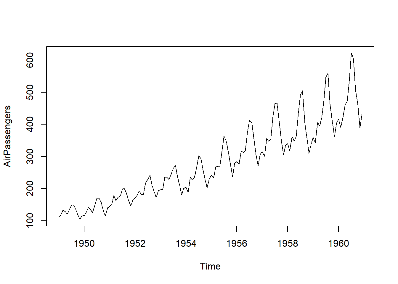
plot.ts(ts_growth_rate_vec(AirPassengers))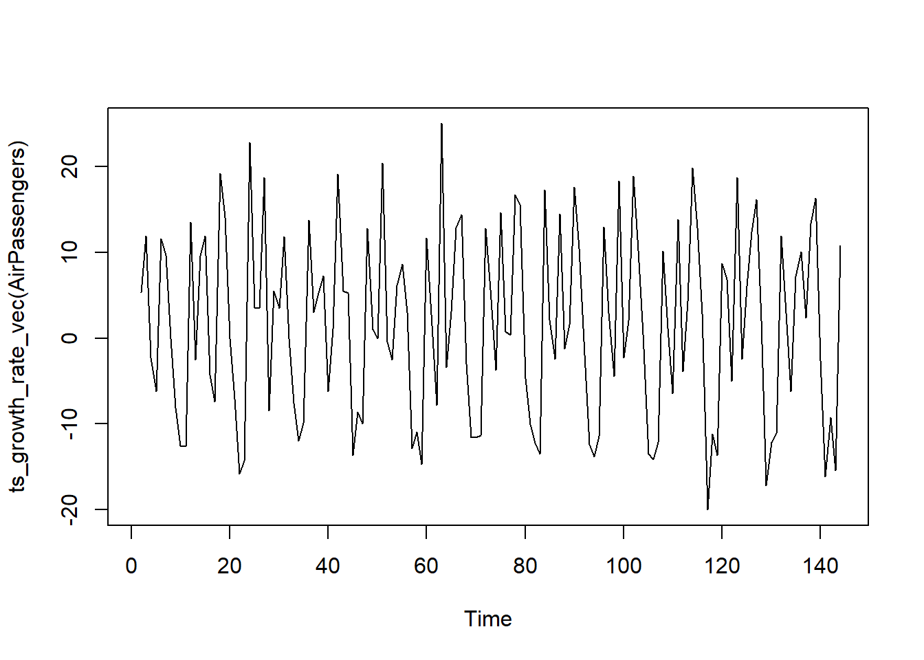
Helper Functions
ts_auto_stationarize
# Example 1: Using the AirPassengers dataset
auto_stationarize(AirPassengers)
The time series is already stationary via ts_adf_test(). Jan Feb Mar Apr May Jun Jul Aug Sep Oct Nov Dec
1949 112 118 132 129 121 135 148 148 136 119 104 118
1950 115 126 141 135 125 149 170 170 158 133 114 140
1951 145 150 178 163 172 178 199 199 184 162 146 166
1952 171 180 193 181 183 218 230 242 209 191 172 194
1953 196 196 236 235 229 243 264 272 237 211 180 201
1954 204 188 235 227 234 264 302 293 259 229 203 229
1955 242 233 267 269 270 315 364 347 312 274 237 278
1956 284 277 317 313 318 374 413 405 355 306 271 306
1957 315 301 356 348 355 422 465 467 404 347 305 336
1958 340 318 362 348 363 435 491 505 404 359 310 337
1959 360 342 406 396 420 472 548 559 463 407 362 405
1960 417 391 419 461 472 535 622 606 508 461 390 432# Example 2: Using the BJsales dataset
auto_stationarize(BJsales)The time series is not stationary. Attempting to make it stationary...Logrithmic Transformation Failed.
Data requires more single differencing than its frequency, trying double
differencing
Double Differencing of order 1 made the time series stationary$stationary_ts
Time Series:
Start = 3
End = 150
Frequency = 1
[1] 0.5 -0.4 0.6 1.1 -2.8 3.0 -1.1 0.6 -0.5 -0.5 0.1 2.0 -0.6 0.8 1.2
[16] -3.4 -0.7 -0.3 1.7 3.0 -3.2 0.9 2.2 -2.5 -0.4 2.6 -4.3 2.0 -3.1 2.7
[31] -2.1 0.1 2.1 -0.2 -2.2 0.6 1.0 -2.6 3.0 0.3 0.2 -0.8 1.0 0.0 3.2
[46] -2.2 -4.7 1.2 0.8 -0.6 -0.4 0.6 1.0 -1.6 -0.1 3.4 -0.9 -1.7 -0.5 0.8
[61] 2.4 -1.9 0.6 -2.2 2.6 -0.1 -2.7 1.7 -0.3 1.9 -2.7 1.1 -0.6 0.9 0.0
[76] 1.8 -0.5 -0.4 -1.2 2.6 -1.8 1.7 -0.9 0.6 -0.4 3.0 -2.8 3.1 -2.3 -1.1
[91] 2.1 -0.3 -1.7 -0.8 -0.4 1.1 -1.5 0.3 1.4 -2.0 1.3 -0.3 0.4 -3.5 1.1
[106] 2.6 0.4 -1.3 2.0 -1.6 0.6 -0.1 -1.4 1.6 1.6 -3.4 1.7 -2.2 2.1 -2.0
[121] -0.2 0.2 0.7 -1.4 1.8 -0.1 -0.7 0.4 0.4 1.0 -2.4 1.0 -0.4 0.8 -1.0
[136] 1.4 -1.2 1.1 -0.9 0.5 1.9 -0.6 0.3 -1.4 -0.9 -0.5 1.4 0.1
$ndiffs
[1] 1
$adf_stats
$adf_stats$test_stat
[1] -6.562008
$adf_stats$p_value
[1] 0.01
$trans_type
[1] "double_diff"
$ret
[1] TRUEConclusion
Ready to jump in? Visit the main page for an overview and to get started with healthyR.ts. The page provides installation instructions, usage examples, and links to detailed documentation to help you hit the ground running.
Functions
library(DT)
library(tidyverse)

# Functions and their arguments for healthyR

pat <- c("%>%",":=","as_label","as_name","enquo","enquos","expr",
         "sym","syms")

tibble(fns = ls.str("package:healthyR.ts")) |>
  filter(!fns %in% pat) |>
  mutate(params = purrr::map(fns, formalArgs)) |>
  group_by(fns) |>
  mutate(func_with_params = toString(params)) |>
  mutate(
    func_with_params = ifelse(
      str_detect(
        func_with_params, "\\("),
      paste0(fns, func_with_params),
      paste0(fns, "(", func_with_params, ")")
    )) |>
  select(fns, func_with_params) |>
  mutate(fns = as.factor(fns)) |>
  datatable(
    #class = 'cell-boarder-stripe',
    colnames = c("Function", "Full Call"),
    options = list(
      autowidth = TRUE,
      pageLength = 10
    )
  )
Join the Community
I encourage you to explore the healthyR.ts package and join the growing community of users. Your feedback and contributions are invaluable in making healthyR.ts a better tool for everyone.
Thank you for your interest, and happy analyzing!
Feel free to reach out if you have any questions or need further assistance. Let’s make time series analysis simpler and more powerful with healthyR.ts!
Best, Steve