Introduction

Today, we’re going to walk through an example of fitting a linear model in R, summarizing the results, and exporting the findings to an Excel file. This workflow is useful for documenting and sharing your statistical analysis.

Let’s break down the code step by step.

Example

Step 1: Loading the Necessary Libraries

First, we need to load the openxlsx library, which helps us create and manipulate Excel files. If you don’t have it installed, you can get it using install.packages("openxlsx").

library(openxlsx)

This line of code loads the openxlsx library into R so we can use its functions later.

Step 2: Fitting the Linear Model

Next, we fit a linear model using the built-in mtcars dataset. We model mpg (miles per gallon) based on all other available variables in the dataset.

model <- lm(mpg ~ ., data = mtcars)

Here, lm stands for linear model. The mpg ~ . part means we want to predict mpg using all other variables in the mtcars dataset.

Step 3: Summarizing the Model

We obtain a summary of our linear model, which includes details like coefficients, R-squared values, and the F-statistic.

model_summary <- summary(model)

This code generates a summary of the linear model we just created, giving us important statistics about the model’s performance.

Step 4: Extracting Key Components

We extract essential parts of the summary for easy access and to organize them in our Excel file.

coefficients <- model_summary$coefficients
r_squared <- model_summary$r.squared
adj_r_squared <- model_summary$adj.r.squared
f_statistic <- model_summary$fstatistic
p_value <- pf(
  f_statistic[1], 
  f_statistic[2], 
  f_statistic[3], 
  lower.tail = FALSE
  )
model_formula <- paste0(
  model_summary[["terms"]][[2]], " ", 
  model_summary[["terms"]][[1]], " ",
  model_summary[["terms"]])[[3]]

coefficients: The estimated coefficients of the model.
r_squared: How well the model explains the variability of the data.
adj_r_squared: Adjusted version of R-squared for the number of predictors.
f_statistic: Overall significance of the model.
p_value: Probability value indicating the significance of the F-statistic.
model_formula: The formula used to fit the model.

Step 5: Creating and Populating the Workbook

Now, we create a new Excel workbook and add a worksheet to it. We then write our extracted model summary components to this worksheet.

wb <- createWorkbook()
addWorksheet(wb, "Model Summary")

writeData(wb, "Model Summary", "Coefficients", 
          startRow = 1, startCol = 1)
writeData(wb, "Model Summary", coefficients, startRow = 2, 
          startCol = 1, rowNames = TRUE)

writeData(wb, "Model Summary", "R-Squared", 
          startRow = 2 + nrow(coefficients) + 2, startCol = 1)
writeData(wb, "Model Summary", r_squared, 
          startRow = 2 + nrow(coefficients) + 2, startCol = 2)

writeData(wb, "Model Summary", "Adjusted R-Squared", 
          startRow = 2 + nrow(coefficients) + 3, startCol = 1)
writeData(wb, "Model Summary", adj_r_squared, 
          startRow = 2 + nrow(coefficients) + 3, startCol = 2)

writeData(wb, "Model Summary", "F-Statistic", 
          startRow = 2 + nrow(coefficients) + 4, startCol = 1)
writeData(wb, "Model Summary", f_statistic[1], 
          startRow = 2 + nrow(coefficients) + 4, startCol = 2)

writeData(wb, "Model Summary", "p-Value", 
          startRow = 2 + nrow(coefficients) + 5, startCol = 1)
writeData(wb, "Model Summary", p_value, 
          startRow = 2 + nrow(coefficients) + 5, startCol = 2)

writeData(wb, "Model Summary", "Model Formula", 
          startRow = 2 + nrow(coefficients) + 6, startCol = 1)
writeData(wb, "Model Summary", model_formula, 
          startRow = 2 + nrow(coefficients) + 6, startCol = 2)

createWorkbook(): Creates a new Excel workbook.
addWorksheet(wb, "Model Summary"): Adds a new sheet named “Model Summary” to the workbook.
writeData: Writes data to the specified location in the sheet. Here, we write various parts of the model summary in different rows and columns.

Step 6: Saving the Workbook

Finally, we save our workbook to a file named lm_model_summary.xlsx.

saveWorkbook(
  wb, 
  file = paste0(getwd(),"/lm_model_summary.xlsx"), 
  overwrite = TRUE
  )

This line saves the workbook to your working directory with the specified file name.

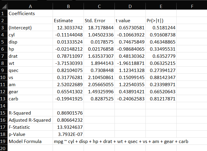
Here is a screenshot:

Conclusion

This example shows how to fit a linear model in R, extract meaningful summary statistics, and save those results in an Excel file. It’s a simple yet powerful way to document your analyses and share them with others.

Feel free to modify the code to fit your own datasets and models. Experimenting with different variables and models can provide deeper insights into your data. Happy coding!