Introduction

If you’re looking for an easy-to-use package to calculate cumulative statistics in R, you may want to check out the TidyDensity package. This package offers several functions to calculate cumulative measurements, including mean, median, standard deviation, variance, skewness, kurtosis, harmonic mean, and geometric mean.

cgmean(): Cumulative Geometric Mean

The cgmean() function calculates the cumulative geometric mean of a set of values. This is the nth root of the product of the first n elements of the set. It’s a useful measurement for sets of values that are multiplied together, such as growth rates.

chmean(): Cumulative Harmonic Mean

The chmean() function calculates the cumulative harmonic mean of a set of values. This is the inverse of the arithmetic mean of the reciprocals of the values. It’s commonly used for sets of values that represent rates, such as speeds.

ckurtosis(): Cumulative Kurtosis

The ckurtosis() function calculates the cumulative kurtosis of a set of values. Kurtosis is a measure of the peakedness of a distribution, relative to a normal distribution. The cumulative kurtosis calculates the kurtosis of a set of values up to a specific point in the set.

cmean(): Cumulative Mean

The cmean() function calculates the cumulative mean of a set of values. It’s a measure of the average of the values up to a specific point in the set.

cmedian(): Cumulative Median

The cmedian() function calculates the cumulative median of a set of values. It’s the value that separates the lower half of the set from the upper half, up to a specific point in the set.

csd(): Cumulative Standard Deviation

The csd() function calculates the cumulative standard deviation of a set of values. Standard deviation is a measure of the spread of values in a set. The cumulative standard deviation calculates the standard deviation up to a specific point in the set.

cskewness(): Cumulative Skewness

The cskewness() function calculates the cumulative skewness of a set of values. Skewness is a measure of the asymmetry of a distribution. The cumulative skewness calculates the skewness up to a specific point in the set.

cvar(): Cumulative Variance

The cvar() function calculates the cumulative variance of a set of values. Variance is a measure of the spread of values in a set. The cumulative variance calculates the variance up to a specific point in the set.

In conclusion, the {TidyDensity} package offers several functions for calculating cumulative statistics, including mean, median, standard deviation, variance, skewness, kurtosis, harmonic mean, and geometric mean. These functions make it easy to calculate cumulative statistics for sets of values in R.

Functions

All of the functions perform work strictly on a vector. Because of this I will not go over the function calls separately because they all follow the vectorized for of fun(.x) where .x is the argument passed to the cumulative function.

Examples

Here I will go over some examples of each function use the AirPassengers data set.

library(TidyDensity)

v <- AirPassengers

Let’s start at the top.

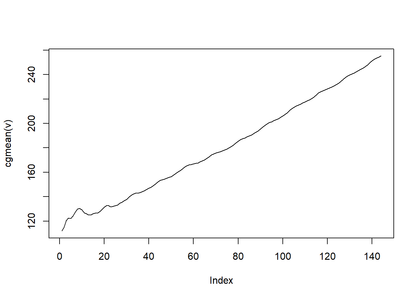
Cumulative Geometric Mean:

head(cgmean(v))

[1] 112.0000 114.9609 120.3810 122.4802 122.1827 124.2311

tail(cgmean(v))

[1] 249.6135 251.1999 252.4577 253.5305 254.2952 255.2328

plot(cgmean(v), type = "l")

Cumulative Harmonic Mean:

head(chmean(v))

[1] 112.00000  57.46087  40.03378  30.55222  24.39304  20.66000

tail(chmean(v))

[1] 1.636832 1.632423 1.627194 1.621471 1.614757 1.608744

plot(chmean(v), type = "l")

Cumulative Kurtosis:

head(ckurtosis(v))

[1]      NaN 1.000000 1.500000 1.315839 1.597316 1.597850

tail(ckurtosis(v))

[1] 2.668951 2.795314 2.733117 2.674195 2.649894 2.606228

plot(ckurtosis(v), type = "l")

Cumulative Mean:

head(cmean(v))

[1] 112.0000 115.0000 120.6667 122.7500 122.4000 124.5000

tail(cmean(v))

[1] 273.1367 275.5143 277.1631 278.4577 279.2378 280.2986

plot(cmean(v), type = "l")

Cumulative Median:

head(cmedian(v))

[1] 112.0 115.0 118.0 123.5 121.0 125.0

tail(cmedian(v))

[1] 259.0 261.5 264.0 264.0 264.0 265.5

plot(cmedian(v), type = "l")

Cumulative Standard Deviation:

head(csd(v))

[1]        NA  4.242641 10.263203  9.358597  8.142481  8.916277

tail(csd(v))

[1] 115.0074 117.9956 119.1924 119.7668 119.7083 119.9663

plot(csd(v), type = "l")

Cumulative Skewness:

head(cskewness(v))

[1]         NaN  0.00000000  0.44510927 -0.14739157 -0.02100016 -0.18544758

tail(cskewness(v))

[1] 0.5936970 0.6471651 0.6349071 0.6145579 0.5972102 0.5770682

plot(cskewness(v), type = "l")

Cumulative Variance:

head(cvar(v))

[1]        NA  18.00000 105.33333  87.58333  66.30000  79.50000

tail(cvar(v))

[1] 13226.70 13922.96 14206.84 14344.08 14330.07 14391.92

plot(cvar(v), type = "l")

Voila!