library(forecast)

data(AirPassengers)
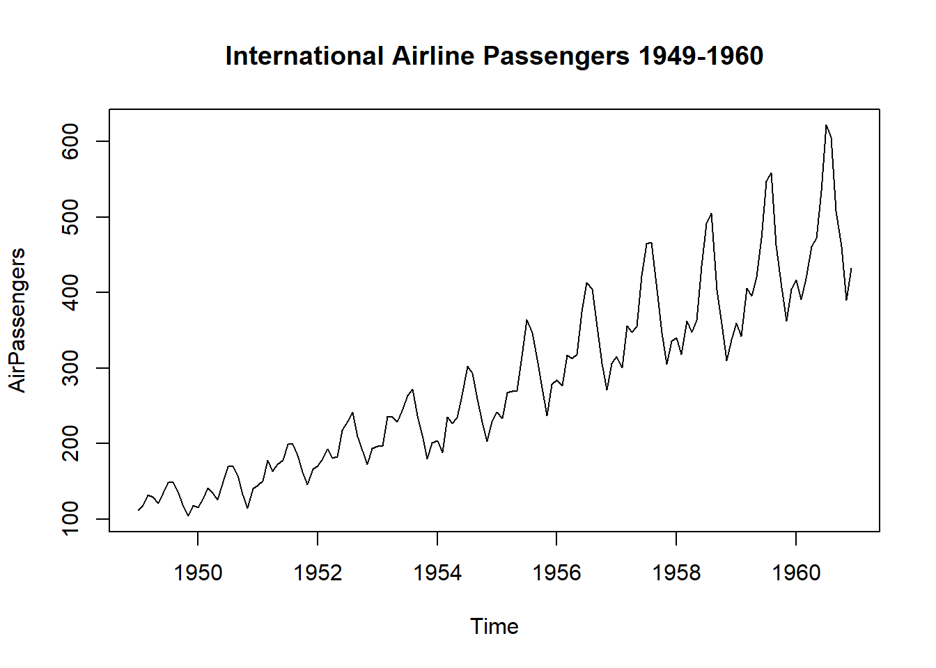
plot(AirPassengers, main = "International Airline Passengers 1949-1960")
Steven P. Sanderson II, MPH
March 29, 2023
Time series analysis is a powerful tool for understanding and predicting patterns in data that vary over time. In this tutorial, we will use the AirPassengers dataset to create a bootstrapped timeseries model in R.
The AirPassengers dataset The AirPassengers dataset contains data on the number of passengers traveling on international flights per month from 1949 to 1960. To begin, we will load the dataset into R and plot it to get an idea of the data’s structure and any underlying patterns.
library(forecast)
data(AirPassengers)
plot(AirPassengers, main = "International Airline Passengers 1949-1960")
From the plot, we can see that there is a clear upward trend in the data, as well as some seasonality.
Now that we have an idea of the structure of the data, we can create a bootstrapped timeseries model using the auto.arima() function from the {forecast} package. The auto.arima() function uses an automated algorithm to determine the best model for a given timeseries.
set.seed(123)
n <- length(AirPassengers)
n_boot <- 1000

# create bootstrap sample indices
boot_indices <- replicate(n_boot, sample(1:n, replace = TRUE))

# create list to store models
models <- list()

# create bootstrapped models
for(i in 1:n_boot) {
  boot_data <- AirPassengers[boot_indices[, i]]
  models[[i]] <- auto.arima(boot_data)
}

models[[1]]
Series: boot_data
ARIMA(0,0,0) with non-zero mean
Coefficients:
mean
275.5347
s.e. 9.5443
sigma^2 = 13209: log likelihood = -887.01
AIC=1778.02 AICc=1778.1 BIC=1783.96In the code above, we first set a seed to ensure reproducibility of our results. We then specify the length of the timeseries and the number of bootstrap iterations we want to run. We create a list to store the models and a set of bootstrap sample indices.
We then loop through each bootstrap iteration, creating a new dataset from the original timeseries by sampling with replacement using the boot_indices. We use the auto.arima() function to create a timeseries model for each bootstrap sample and store it in our models list.
Now that we have created our bootstrapped timeseries models, we can summarize and plot the residuals of each model to get an idea of how well our models fit the data.
# create list to store residuals
residuals <- list()

# create residuals for each model
for(i in 1:n_boot) {
  boot_data <- AirPassengers[boot_indices[, i]]
  residuals[[i]] <- residuals(models[[i]])
}

# summarize residuals
residual_means <- sapply(residuals, mean)
residual_sd <- sapply(residuals, sd)

# plot residuals
par(mfrow = c(2, 1))

hist(
  residual_means,
  main = "Bootstrapped Model Residuals",
  xlab = "Mean Residuals"
  )
hist(
  residual_sd,
  col = "red",
  main = "",
  xlab = "SD Residuals"
  )
In the code above, we create a list to store the residuals for each model, loop through each model to create residuals using the residuals() function, and summarize the residuals by taking the mean and standard deviation of each set of residuals.
We then plot the mean residuals and standard deviations for each model using the plot() function and add a legend to indicate the meaning of the two lines.
Voila!